Create an End to End Streaming Pipeline with Kafka, Docker, Confluent, Mage, BigQuery and dbt

Table of Contents

• Set-up Google Platform, a Virtual Machine and Connect to it Remotely through Visual Studio Code
  • Create a Google Cloud Project
  • Create a Virtual Machine
  • Create SSH Keys and Access VM Remotely
  • Access VM Through Visual Studio Code (VS Code)
• Stream from UK’s Companies House API and Produce to Kafka
  • Create a GitHub Repository
  • Stream data from UK’s Companies House
  • What’s Kafka
  • Create a Kafka Cluster
  • Produce Simulated Data to a Kafka Topic
  • Produce UK’s Companies House Data to a Kafka Topic
• Containerize our Application
  • Create a Docker Container of our Application
• From Kafka to BigQuery through Mage
  • Install Mage
  • Consume Data from Kafka Topic
  • Send Streamed Data to BigQuery
  • Create Table that Contains all UK’s Companies House Data
• Apply Transformations with dbt (data build tool)
  • How to Set-Up dbt
  • Create dbt Data Sources
  • Create dbt Models
  • Test the Entire Pipeline in a Development Environment
  • Test the Pipeline in Production
  • Schedule and Run the Entire Pipeline

Goal of the Project and Explanation

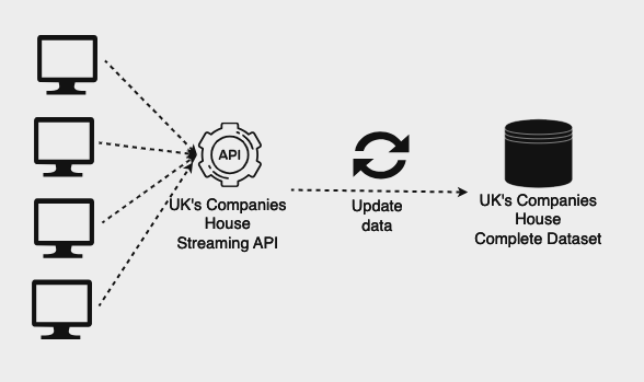
This guide aims to achieve two goals: stream data in real-time from UK’s Companies House and integrate it with the entire dataset as new data becomes available over time.

The UK Companies House is an executive agency of the UK Government, responsible for incorporating and dissolving limited companies, registering company information, and making this information available to the public.

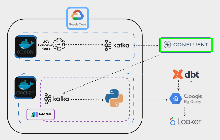
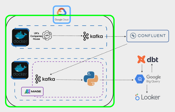
Here is a simplified architecture of the project:

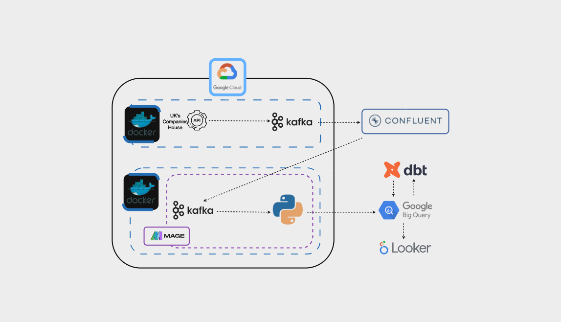
Here is the technical architecture:

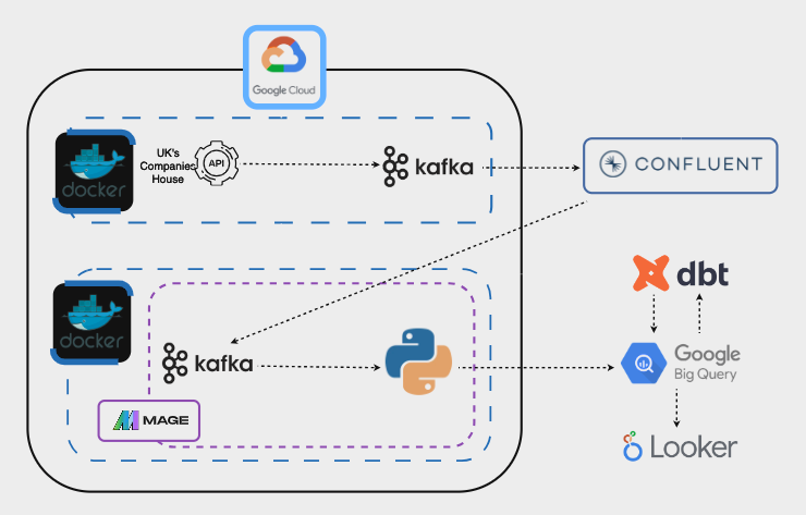
Let’s go through the different steps.

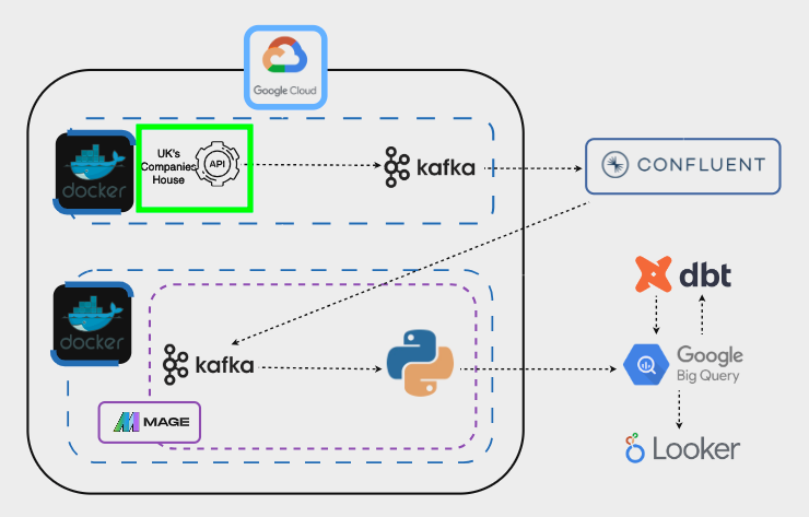
The first task is actually being able to stream data from UK’s Companies House API:

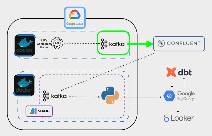
Once we are able to do this, we need to create a Kafka cluster on Confluent to serve as the intermediary for the streaming data:

Afterwards, we’ll create a Kafka producer, a mechanism for streaming data to Kafka clusters:

All of the previous steps involve several scripts and multiple packages. To simplify the deployment and mitigate dependency issues we’ll encapsulate all components into a Docker container. In this way, we’ll be to able to stream data to our Kafka cluster with one simple line of code, docker start container_id.

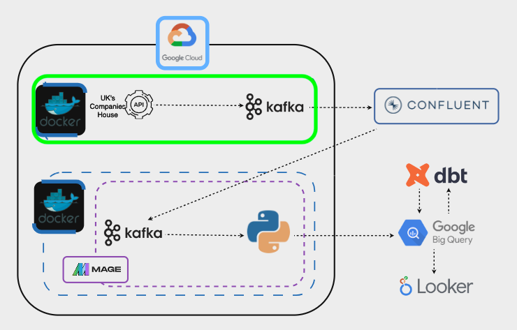
Our Docker containers will be within a virtual machine, because we want to run them 24/7. If we run them locally, as soon as we shut down our computer, the containers will also stop:

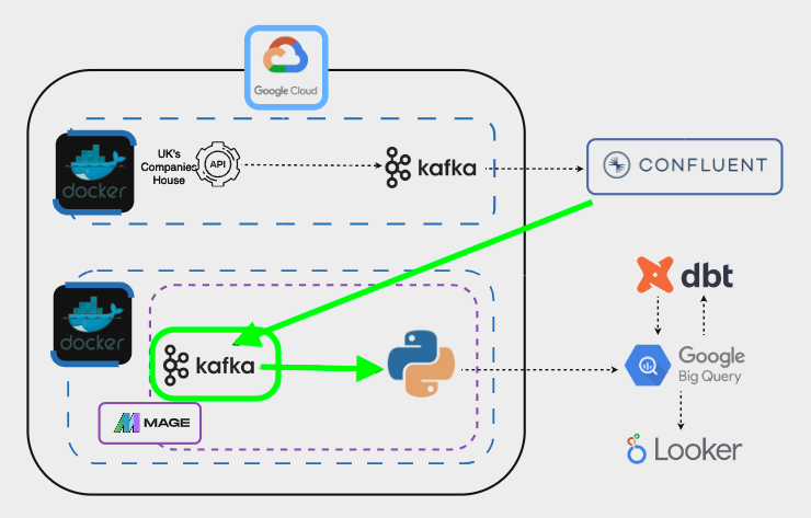
To retrieve the flow of data from Kafka and forward it to downstream processes, we’ll use Mage as an orchestrator. To ensure continuous operation, Mage we’ll also be encapsulated in a Docker container:

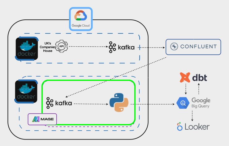
In Mage, the initial block will consume data from the Kafka Cluster and pass it to a Python script:

This script will conduct an initial cleanup of the data and then stream it in real-time to BigQuery:

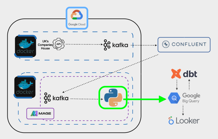
In BigQuery, initially we’ll manually upload the entire dataset from the UK’s Companies House. Afterwards, we’ll utilize dbt (data build tool) to incrementally update the dataset with streaming data as it becomes available:

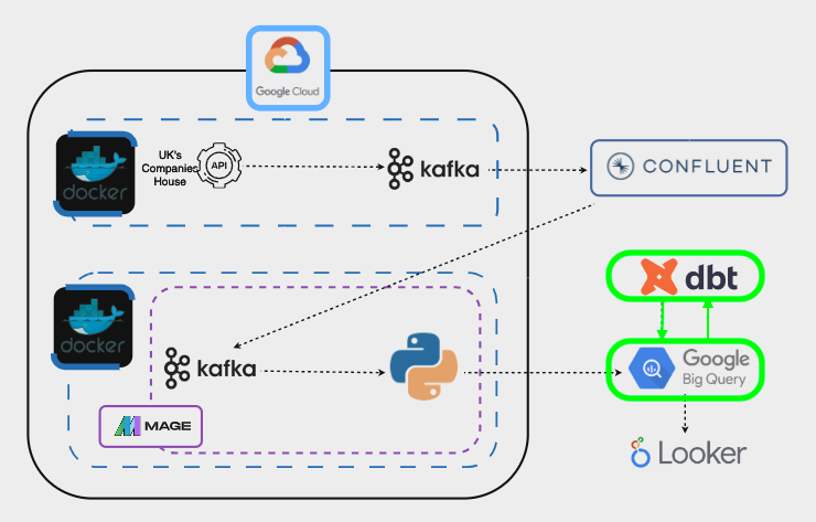
Finally, we can visualize the data with our BI tool of preference. However, this will not be covered in this guide.

The GitHub repository is available here.

Set-up Google Platform, a Virtual Machine and Connect to it Remotely through Visual Studio Code

Create a Google Cloud Project

The first thing that we have to do is to create a GCP project. In this project we’ll host many of the things that we’ll build, such as the application to produce streaming data, our orchestration tool, Mage, as well as our BigQuery database.

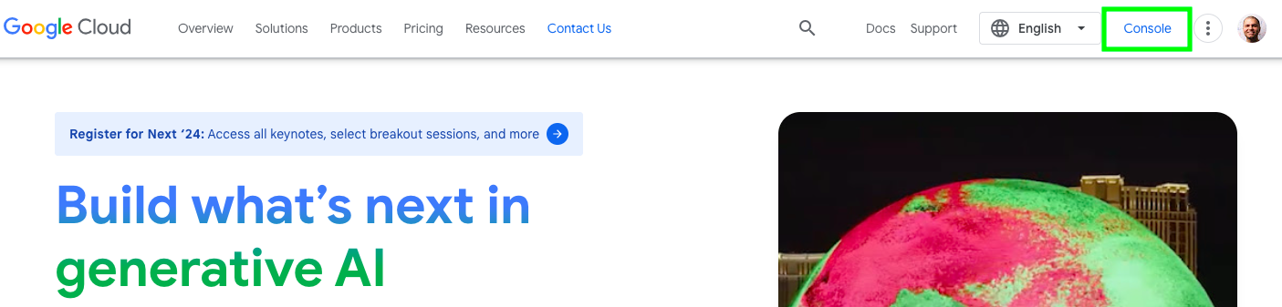
Once you reach the Google Cloud Homepage, click on Console on the top right corner.

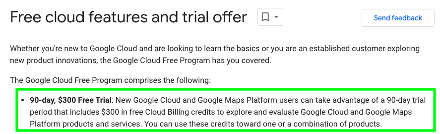
If you have never been a paying customer of Google Cloud, you should be able to enjoy a $300 free credit.

Once you are in the console, click on the top left, next to the Google Cloud logo.

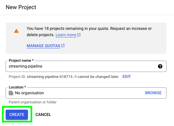
Then, on the top right, click on NEW PROJECT

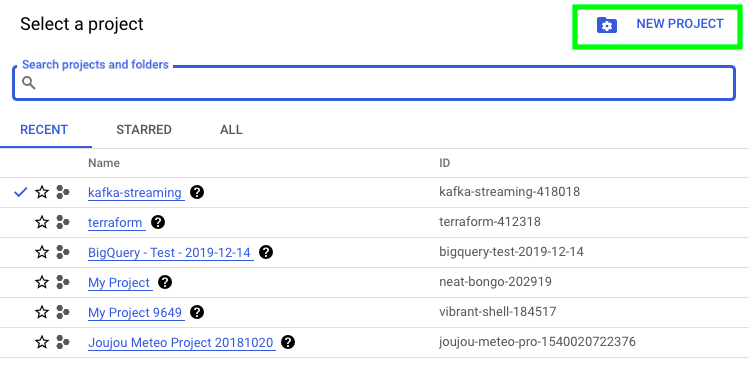
Give your project a name and click on CREATE. I’ll call mine streaming-pipeline:

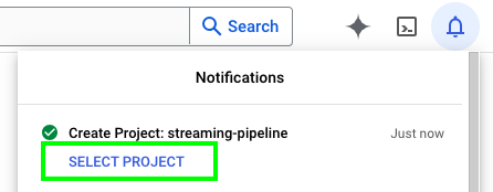
Once your project has been created, click on SELECT PROJECT:

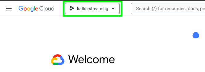
Now, at the top left corner, you should see the name of your project:

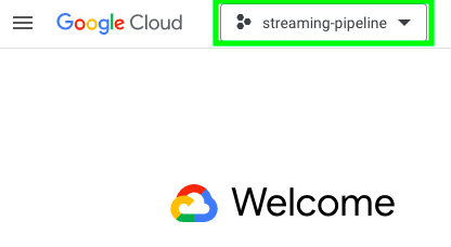
Now, let’s move to the next step, creating a virtual machine.

Create a Virtual Machine

A virtual machine is essentially a computer within a computer. For instance, you can create a virtual machine on your local computer, completely separate from the physical hardware. In our case, we’re opting to create a virtual machine in the cloud. Why? Because that’s where our orchestrator, Mage, will reside. We need to host Mage on a machine that never shuts down to ensure the streaming pipeline can run continuously.

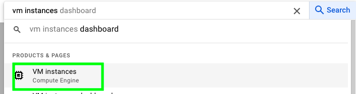
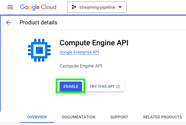
To create a virtual machine (VM), type vm instances in the search bar and click on VM instances:

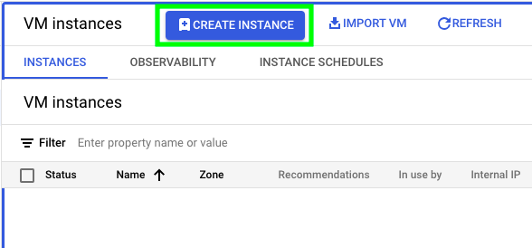
This will take you to a screen where you’ll see the option to enable the Compute Engine API. In Google Cloud, enabling specific services is akin to loading libraries in programming languages. In our case, we need the Compute Engine API to create and run a VM. Click on ENABLE to proceed:

Once the API has finished loading, click on CREATE INSTANCE:

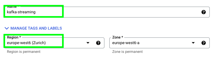
Give your VM a name and choose the region closest to you. Remember, we’ll be creating other services later on. It’s essential to maintain consistency in the region selection. Otherwise, when different services need to interact, they may encounter issues if their data is located in different regions.

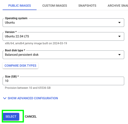
Go to the Boot disk section and click on CHANGE:

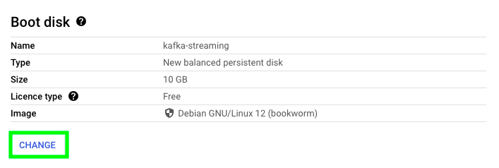
Select the following options and click on SELECT:

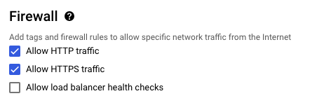
Under Firewall select the following options. We need to enable these options otherwise we won’t be able to access Mage from the outside world.

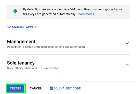
Now, click on CREATE:

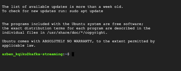
Once you VM is created, you can click on SSH to access it:

If everything works properly, you should see a screen similar to this:

Congratulations, you’ve successfully accessed your VM! However, working with the VM directly from the browser can be inconvenient, as it lacks the benefits of a modern IDE like Visual Studio Code. Therefore, we need to find a way to connect to our VM remotely. This is where SSH keys come in.

Create SSH Keys and Access VM Remotely

SSH keys are a mechanism that allows you to securely connect to third-party applications. When you create SSH keys, you have two of them:

• A public SSH key, which you share with third-party applications - think of it as the lock
• A private SSH key, which you keep on your machine - think of it as the key

In essence, on your machine, you have the key to open the lock. When you open the lock, you access the third-party application. On a side note, I think that calling SSH keys both keys is a bit misleading. I would have personally called them SSH key and SSH lock. This would have made things easier to understand.

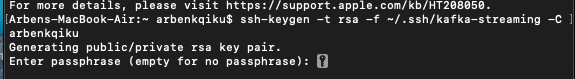
Anyway, go to your terminal, and type the following:

 ssh-keygen -t rsa -f ~/.ssh/kafka-streaming -C arbenkqiku

In this case, kafka-streaming is the name that we give to our keys, and arbenkqiku is my username. If you don’t know your username, simply type:

whoami

Add a password to your SSH keys. This is an additional security measure to prevent unwanted access.

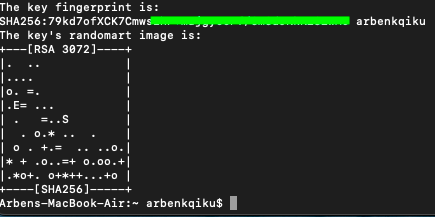
This will create your SSH keys:

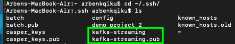
To locate your SSH keys, go to the following directory:

cd ~/.ssh/

If you type the following command, you’ll see the content of your directory:

ls

You should be able to see the keys that we have just created. Please store them securily.

Now, we need to take our public key, the lock, and add it to our VM.

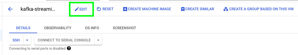
Go to where your VM is located, and click on its name:

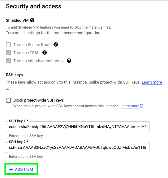
Click on EDIT:

Go to the section called Security and access, and click on ADD ITEM:

Now, go back to the terminal and type:

cat kafka-streaming.pub

This will display the content of your public key, your lock.

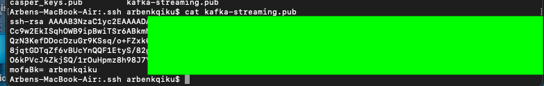
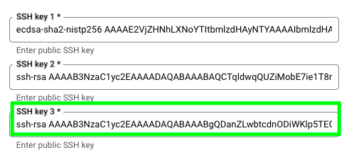
Copy the content of your public key and add it to your VM:

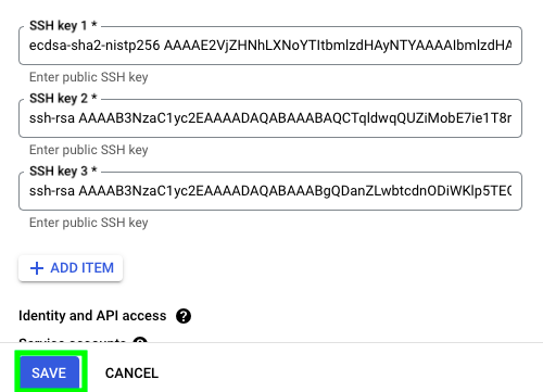
Click on SAVE:

Now, go back to where your VM is located and copy the External IP address. This basically represents the location of your VM.

Go back to terminal and type:

ssh -i kafka-streaming arbenkqiku@34.65.113.154

Here is what the previous command means:

ssh -i name_of_private_key user_name@gcp_vm_instance_external_ip

With this command, we are basically saying: go to this external IP address, and use this private key to acces the VM. Once you run the command, it will ask you if you are sure you want to connect, type yes. You’ll also be prompted to add the password that we added to the SSH keys when we created them.

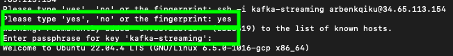
If everything worked correctly, you should be inside your VM:

Access VM Through Visual Studio Code (VS Code)

Now that we know that we can access our VM remotely, let’s do the same thing through VS code. Go to this link and download VS code.

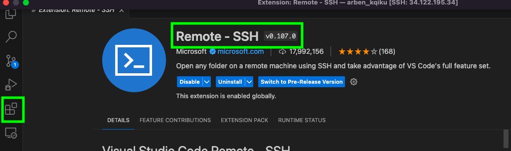
Then, go to extensions, look for remote ssh and install the “Remote - SSH” extension:

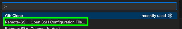
In VS code, go to the the search bar and type > and select the following option:

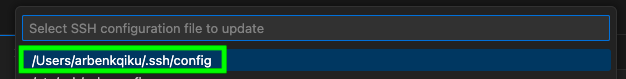
If you already have an SSH config file, select it:

Then, type the following:

Host kafka-streaming # Give a name to your host, this could be anything you want
  HostName 34.65.113.154 # Replace with the External IP address in GCP
  User arbenkqiku # Replace this with your user name
  IdentityFile /Users/arbenkqiku/.ssh/kafka-streaming # Location of your private SSH Key

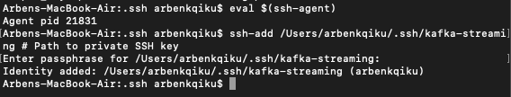
Now, we still have to go back to the terminal one last time and type this:

eval $(ssh-agent)
ssh-add /Users/arbenkqiku/.ssh/kafka-streaming # Path to private SSH key

Then, type your password when prompted. This basically means that you can use your password when you try to access the VM through Visual Studio Code.

Now, go back to the search bar of Visual Studio Code, type > and select the following option:

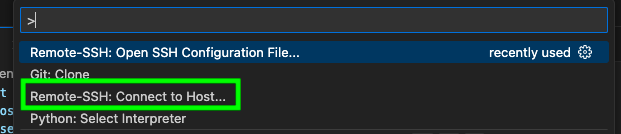
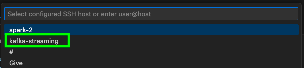
Among the options, you should see the host that you just created. Click on it:

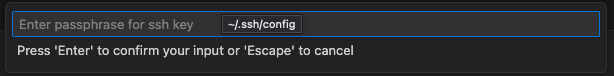
This should open a new window and you should be prompted to add your password:

In the new window, click on this icon at the top right to open the terminal in VS code:

First of all, we can can see our user name followed by the name of the VM:

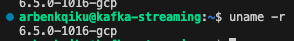
In addition, if we type:

uname -r

We can see that it is a GCP (Google Cloud Platform) machine.

Congrats! We connected to the VM remotely by using VS code.

Stream from UK’s Companies House API and Produce to Kafka

Create a GitHub Repository

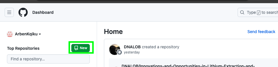
Let’s create a GitHub repository where we’ll store all of our code. Go to GitHub and click on NEW:

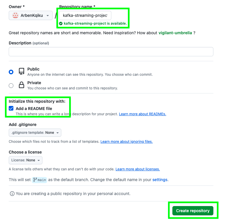
Give your repo a name, select the Add a README file checkbox and click on Create repository:

Now, click on Code and copy the URL of the repo:

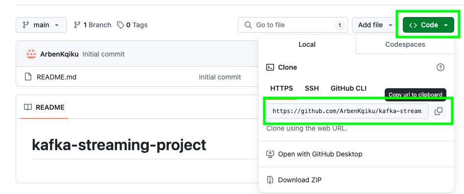
Go to the terminal of your VM in VS code and type:

git clone https://github.com/ArbenKqiku/kafka-streaming-project.git

This will clone our project locally. Now, we can make changes locally and push them to our repository.

Stream Data from UK’s Companies House

So, our goal right now will be to create a python script able to stream data in real time from UK’s Companies House streaming API. Here the steps that we’ll have to follow:

• Register an account on the API
• Create an application

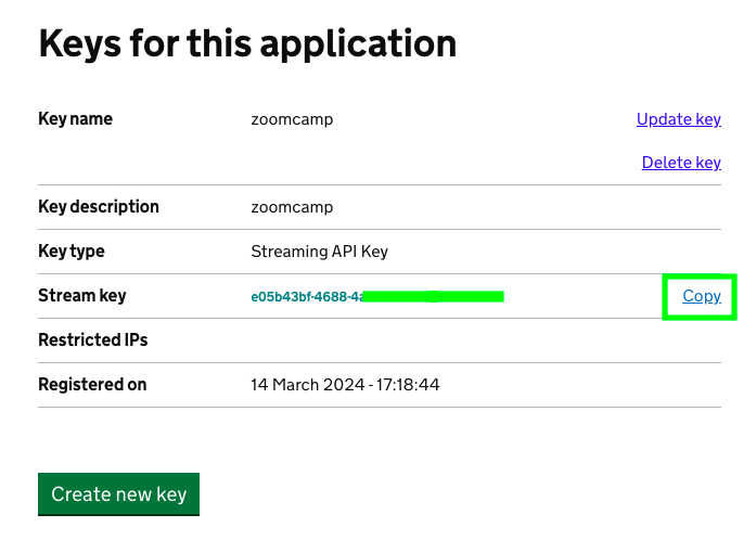
Once you have created the application, you can click on it:

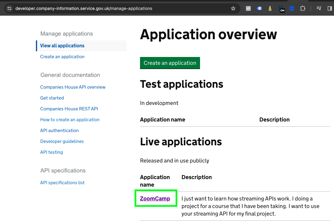
Copy the API key and store it somewhere:

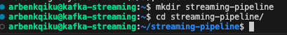
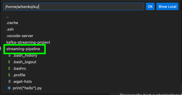
In the terminal, create a directory named streaming-pipeline and access it.

Now that you have created the directory, click on Open…:

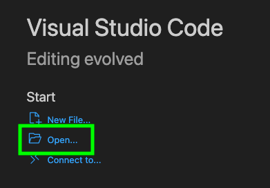
You should see that directory that we just created. Click on it:

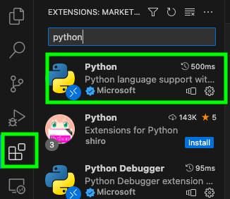
You’ll prompted to enter your password again. Now, let’s install the python extention. This will make it easier to code later on. Go to Extensions and install the Python extension.

Now, we need to install pip in order to install python libraries. Go to the terminal and type the follwing command:

sudo apt update

The sudo apt update command is used on Debian-based Linux systems, such as Ubuntu, to update the package lists for repositories configured on the system.

Then type the following to install pip:

sudo apt install python3-pip

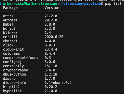
If you type:

pip list

You should be able to see python packages installed by default:

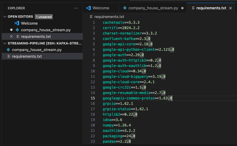
Here is the list of packages that we’ll have to install to complete the project. Copy them and save them into a file named requirements.txt

cachetools==5.3.3
certifi==2024.2.2
charset-normalizer==3.3.2
confluent-kafka==2.3.0
google-api-core==2.18.0
google-api-python-client==2.123.0
google-auth==2.29.0
google-auth-httplib2==0.2.0
google-auth-oauthlib==1.2.0
google-cloud==0.34.0
google-cloud-bigquery==3.19.0
google-cloud-core==2.4.1
google-crc32c==1.5.0
google-resumable-media==2.7.0
googleapis-common-protos==1.63.0
grpcio==1.62.1
grpcio-status==1.62.1
httplib2==0.22.0
idna==3.6
numpy==1.26.4
oauthlib==3.2.2
packaging==24.0
pandas==2.2.0
proto-plus==1.23.0
protobuf==4.25.3
pyarrow==15.0.0
pyasn1==0.5.1
pyasn1-modules==0.3.0
pyparsing==3.1.2
python-dateutil==2.8.2
pytz==2024.1
requests==2.31.0
requests-oauthlib==2.0.0
rsa==4.9
six==1.16.0
tzdata==2023.4
uritemplate==4.1.1
urllib3==2.2.1

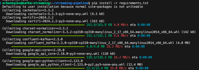
Then, install all the packages with this command:

pip install -r requirements.txt

This should start the installation:

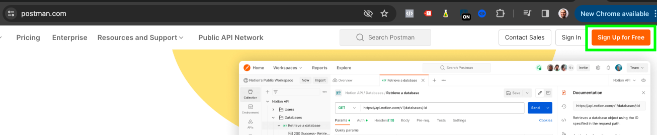
Now, we need to test our API connection. Before testing it in the code, I usually prefer to test things in Postman. Postman is a platform that simplifies the process of working with APIs by providing a user-friendly interface for sending HTTP requests and viewing their responses. Go to the link previously provided and create an account:

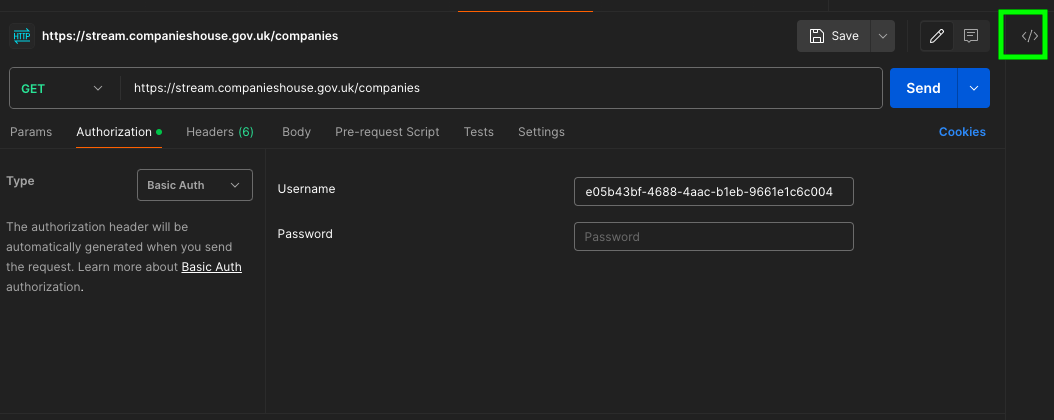
Once you are in Postman, type https://stream.companieshouse.gov.uk/companies in the request field:

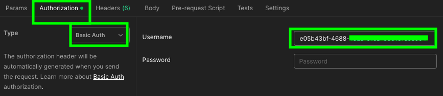
Go to Authorization, select Basic Auth and under Username paste your API key.

In theory, this should not work, but I could not find any alternatives. Usually, you simply add the API key at the end of the URL, similar to this:

https://stream.companieshouse.gov.uk/companies?api_key=12345

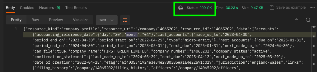
However, this was the only way to make it work. If everything worked correctly, the status of the request should indicate 200 OK and you should some results:

Please note that the response may take some time. In my experience, it could take approximately 30 seconds. Occasionally, the cloud agent of Postman may not function properly when a request exceeds this duration. In such cases, you can try sending the request multiple times (I had to do it up to 3 times). Alternatively, consider downloading Postman Desktop, which has a higher tolerance for lengthier requests.

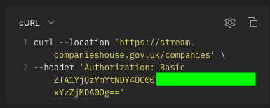
Postman makes it super easy to build your API requests. Once you have built a successful request, you can translate it to actual code in multiple programming languages. I love this feature of Postman. To see what our request looks in code, click on this icon at the top right:

You’ll see that the Authorization header looks different than the API key. In reality, it is a Base64-encoded representation of the API.

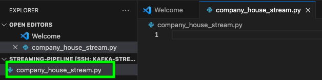
Now, let’s go back to the terminal in VS code. Click this icon to create a new file:

Name the file company_house_stream.py and click on enter:

Here is the code to create the API request:

import requests
import json

# Define the base URL for the Companies House API
base_url = "https://stream.companieshouse.gov.uk/"

# Make a GET request to the 'companies' endpoint
response = requests.get(
    url=base_url + "companies",
    headers={
        "Authorization": 'Basic faefaefae==',
        "Accept": "application/json",
        "Accept-Encoding": "gzip, deflate"
    },
    stream=True  # Stream the response data
)

First of all, we’re importing the necessary packages. Then, we define the endpoint with the necessary headers, that we got from Postman. Even though my request is exactly the same as in Postman, for some reason it would not work. I later discovered that the issue is due to the stream argument. When accessing a streaming API, it is very important to specifiy this aspect. With the previous code, our request is successful, however, it doesn’t produce any output. We need to find a way to create an open connection, where results are streamed and displayed in real time.

Let’s add this piece of code:

# Stream data as it comes in
for line in response.iter_lines():
    # if there is data, decode it and convert it to json.
    if line:
        decoded_line = line.decode('utf-8')

        json_line = json.loads(decoded_line)

        # print streamed line
        print(json_line)

With this piece of code for line in response.iter_lines():, we iterate over each line of data received from the response object. iter_lines() is a method provided by the requests library to iterate over the response content line by line. With if line: we check for data. With if line: decoded_line = line.decode('utf-8'), if there is data in the line, it is decoded from bytes to a string using UTF-8 encoding. The decode() method is used to decode byte sequences into strings. With json_line = json.loads(decoded_line), once the line of data is decoded, it is assumed to be in JSON format, and the loads() method from the json module is used to parse the JSON data into a Python dictionary. Finally, it is printed. this is the final code:

import requests
import json

url = "https://stream.companieshouse.gov.uk/"

response=requests.get(
    url=url+"companies",
    headers={
        "Authorization": 'Basic ZTA1YjQzYmYtNabcabcabcabcabcabcabcabcabcabc',
        "Accept": "application/json",
        "Accept-Encoding": "gzip, deflate"
    },
    stream=True
)

print("Established connection to Company House UK streaming API")

for line in response.iter_lines():
    if line:
        decoded_line = line.decode('utf-8')

        json_line = json.loads(decoded_line)

        print(json_line)

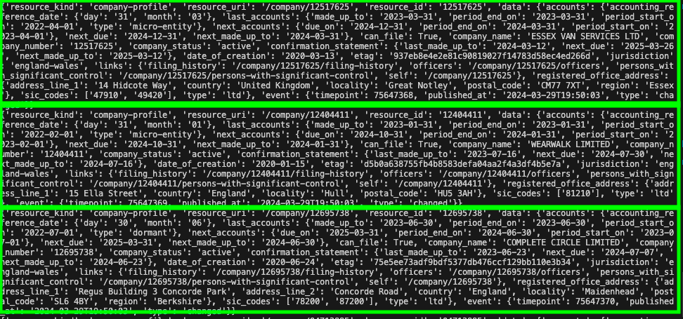
If everything works correctly, you should have an open connection to the API and see continuosly streamed data:

However, let’s try to make our code more resistant by handling exceptions:

import requests
import json

url = "https://stream.companieshouse.gov.uk/"

try:
    response=requests.get(
        url=url+"companies",
        headers={
            "Authorization": 'Basic ZTA1YjQzabcabcabcabcabcabcabcabcabcabc',
            "Accept": "application/json",
            "Accept-Encoding": "gzip, deflate"
        },
        stream=True
    )

    print("Established connection to Company House UK streaming API")

    for line in response.iter_lines():
        if line:
            decoded_line = line.decode('utf-8')

            json_line = json.loads(decoded_line)

            # Build empty JSON
            company_profile = {
                "company_name": None,
                "company_number": None,
                "company_status": None,
                "date_of_creation": None,
                "postal_code": None,
                "published_at": None
            }

            try:
                company_profile['company_name'] = json_line["data"]["company_name"]
            except KeyError:
                company_profile['company_name'] = "NA"

            try:
                company_profile['company_number'] = json_line["data"]["company_number"]
            except KeyError:
                company_profile['company_number'] = "NA"
            
            try:
                company_profile['company_status'] = json_line["data"]["company_status"]
            except KeyError:
                company_profile['company_status'] = "NA"

            try:
                company_profile["date_of_creation"] = json_line["data"]["date_of_creation"]
            except KeyError:
                company_profile["date_of_creation"] = "NA"

            try:
                company_profile["postal_code"] = json_line["data"]["registered_office_address"]["postal_code"]
            except KeyError:
                company_profile["postal_code"] = "NA"

            try:
                company_profile["published_at"] = json_line["event"]["published_at"]
            except KeyError:
                company_profile["published_at"] = "NA"

            print("")
            print("BREAK")
            print("")
            print(company_profile)

except Exception as e:
    print(f"an error occurred {e}")

Firstly, it’s essential to handle exceptions that may occur when connecting to the API. Additionally, while the API provides a lot of columns for each row, we are only interested in retrieving specific fields. To facilitate this, I’ve initialized an empty JSON placeholder:

# Build an empty JSON placeholder
company_profile = {
    "company_name": None,
    "company_number": None,
    "company_status": None,
    "date_of_creation": None,
    "postal_code": None,
    "published_at": None
}

Then, I attempt to access the desired fields using try-except blocks:

try:
    # Check if the key 'company_name' exists in json_line. If it does, assign its value to the 'company_name' key in the company_profile dictionary.
    company_profile['company_name'] = json_line["data"]["company_name"]
except KeyError:
    # If the key does not exist, assign "NA" to the 'company_name' key in the company_profile dictionary.
    company_profile['company_name'] = "NA"

As you can see, for each company data that we stream, we only keep the data we’re interested:

As the next step, we’ll stream our data to Kafka!

What is Kafka?

Apache Kafka is a streaming platform that is used for building real-time data pipelines and streaming applications. In simple terms, think of Apache Kafka as a large messaging system that allows different applications to communicate with each other by sending and receiving streams of data in real-time. Apache Kafka was originally developed by engineers at LinkedIn. Kafka was conceived to address the challenges LinkedIn faced in handling real-time data streams, such as user activity tracking, operational metrics, and logging. In 2011, Kafka was open-sourced and became an Apache Software Foundation project.

In Kafka, there are essentially producers and consumers of data.

However, the data is not directly shared from a producer to a consumer. The producer first sends the data to a topic, and then the consumer retrieves this data from the topic.

In our project, there will only one consumer, but in reality, there could be multiple consumers retrieving data from a topic:

One of the strengths of Kafka is that each topic can have multiple copies, called partitions.

Think of a Kafka partition as a separate stack of ordered messages within a library. Each stack (partition) holds a series of messages related to a particular topic. This has many advantages:

1. Parallel Work: If multiple people want to read different books, they have to wait for their turn. Now, imagine if there are several stacks of books (partitions). Different people can read different books at the same time without waiting.

2. Scalability: Let’s say the library gets more popular, and more books keep coming in. Instead of piling them all on one stack (partition), we create more stacks. This way, each stack can handle its own set of books without getting too crowded.

3. Reliability: What if one of the book stacks falls over or gets damaged? If all the books were in that one stack, it would be a problem. But since we have multiple stacks (partitions), if something happens to one, the others are still okay.

Kafka partitions are within a broker. A Kafka broker is a single server instance within the Kafka cluster. Brokers store and manage data (partitions) and handle requests from producers and consumers. Imagine a librarian at a specific desk in the library. Each librarian (broker) manages a set of books (partitions) and assists library visitors (producers and consumers).

A Kafka cluster is a collection of Kafka brokers that work together to handle and manage the flow of messages. Think of the Kafka cluster as a team of librarians working together in a large library.

Create a Kafka Cluster

To send messages to Kafka, we first need to create a Kafka Cluster. To do that, we’ll use Confluent. Confluent is a company founded by the creators of Apache Kafka. Confluent abstracts the complexities of managing Kafka clusters, similar to how Google Cloud abstracts the underlying server infrastructure for cloud-based services.

Once you are on the homepage, click on GET STARTED FOR FREE and create an account:

If you are new to Confluent, you get a $400 credit:

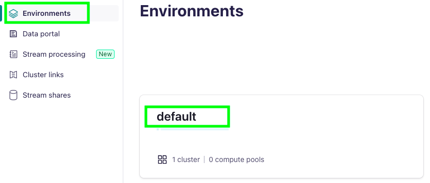
Click on Environments and then on default:

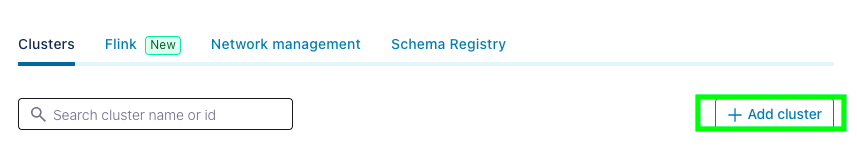
Click on Add cluster:

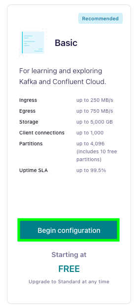
Select the Basic plan and click on Begin configuration:

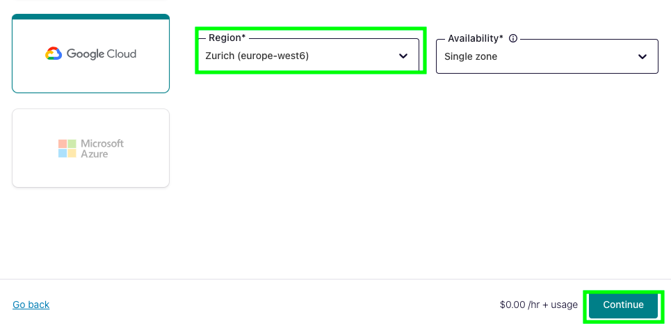
Select a region and click on Continue:

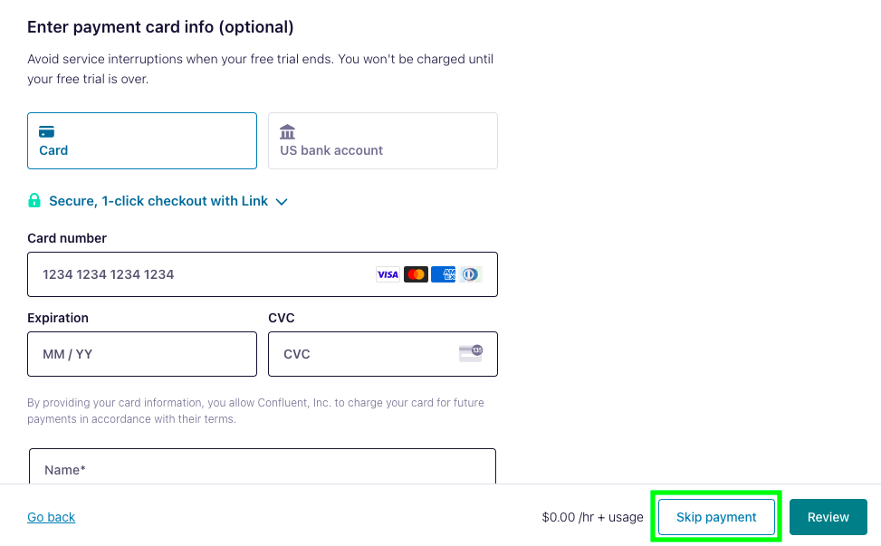
Click on Skip payment. Be aware that you need to add a credit card if you don’t want your application to stop after you run out of the free credit:

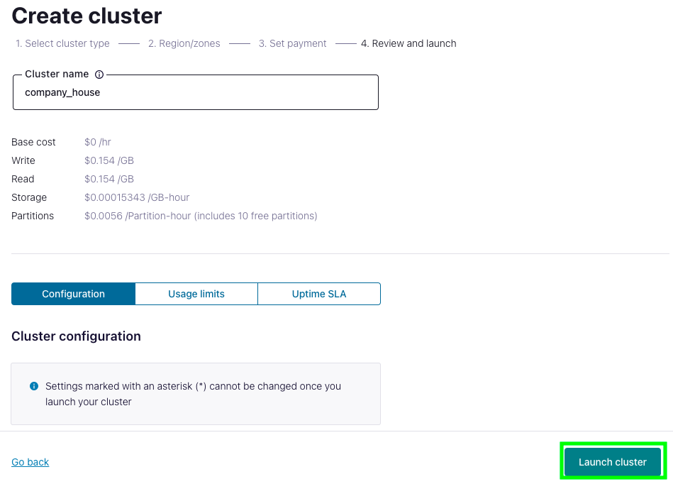
Give a name to your cluster and click on Launch cluster:

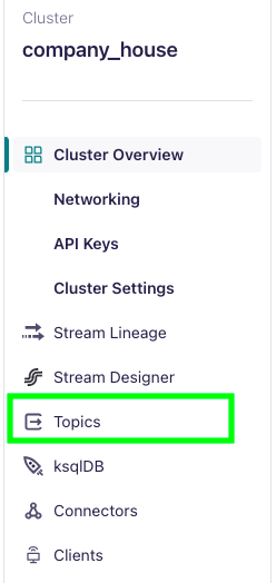
Click on Topics:

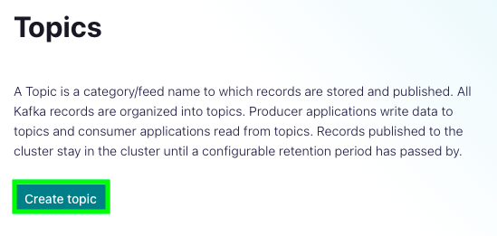
Click on Create topic:

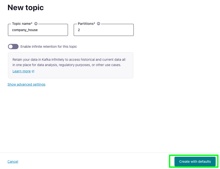
Give you topic a name, I named mine company_house, and select 2 partitions, which are more than sufficient for our project. Then, click on Create with defaults:

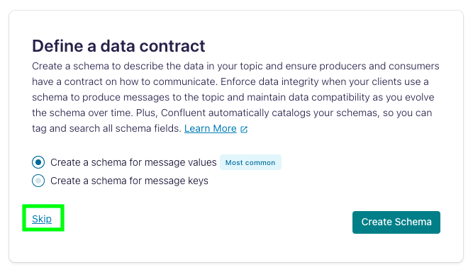
You can also define a data contract, but we’ll skip this step:

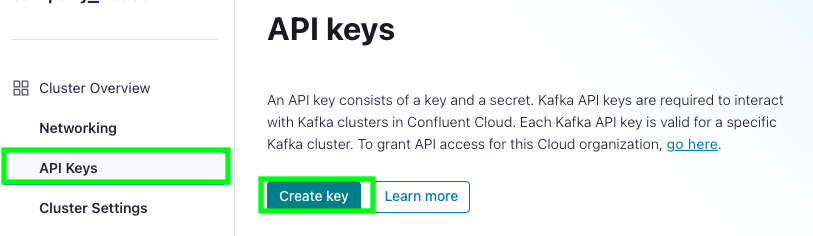
Now that our topic is created, go to API keys and click on Create key:

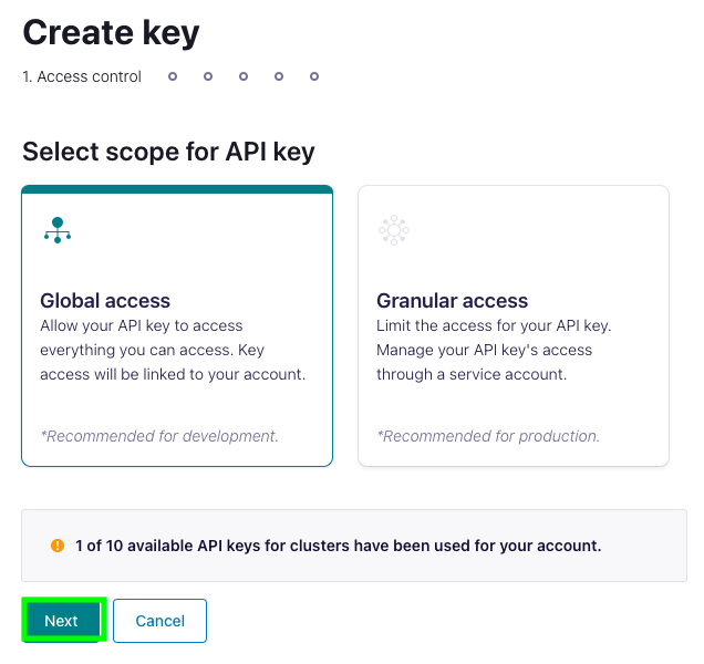
Select the Global access option and click on Next:

Click on Download and continue and store your API Key and Secret somewhere safe:

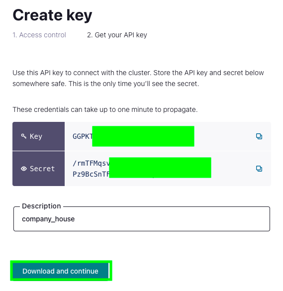
We’re all set, we can now start producing data to our Kafka topic!

Produce Simulated Data to a Kafka Topic

I have taken part the following guide from Confluent’s documentation. To produce data to our Kafka cluster, we need a configuration file. In the VM, copy and paste the following configuration data into a file named getting_started.ini, substituting the API key and secret that you just created for the sasl.username and sasl.password values, respectively.

[default]
bootstrap.servers=
security.protocol=SASL_SSL
sasl.mechanisms=PLAIN
sasl.username=< CLUSTER API KEY >
sasl.password=< CLUSTER API SECRET >

[consumer]
group.id=python_example_group_1

# 'auto.offset.reset=earliest' to start reading from the beginning of
# the topic if no committed offsets exist.
auto.offset.reset=earliest

To find your bootstrap server, go under Cluster Settings:

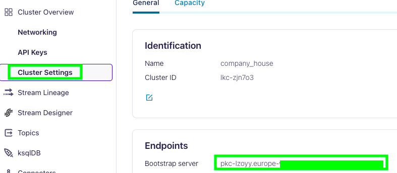
Here is what it should look like:

[default]
bootstrap.servers=pkc-lzoyy.europe-west6.abcabcabcabcabc
security.protocol=SASL_SSL
sasl.mechanisms=PLAIN
sasl.username=GGPabcabcabcabcabc
sasl.password=/rmTFMqsvD4/CEs7tJEZAD6/NV9OOabcabcabcabcabcabcabcabcabcabc

[consumer]
group.id=python_example_group_1

# 'auto.offset.reset=earliest' to start reading from the beginning of
# the topic if no committed offsets exist.
auto.offset.reset=earliest

Now, create a file named producer.py and paste the following:

#!/usr/bin/env python

import sys
from random import choice
from argparse import ArgumentParser, FileType
from configparser import ConfigParser
from confluent_kafka import Producer

if __name__ == '__main__':
    # Parse the command line.
    parser = ArgumentParser()
    parser.add_argument('config_file', type=FileType('r'))
    args = parser.parse_args()

    # Parse the configuration.
    # See https://github.com/edenhill/librdkafka/blob/master/CONFIGURATION.md
    config_parser = ConfigParser()
    config_parser.read_file(args.config_file)
    config = dict(config_parser['default'])

    # Create Producer instance
    producer = Producer(config)

    # Optional per-message delivery callback (triggered by poll() or flush())
    # when a message has been successfully delivered or permanently
    # failed delivery (after retries).
    def delivery_callback(err, msg):
        if err:
            print('ERROR: Message failed delivery: {}'.format(err))
        else:
            print("Produced event to topic {topic}: key = {key:12} value = {value:12}".format(
                topic=msg.topic(), key=msg.key().decode('utf-8'), value=msg.value().decode('utf-8')))

    # Produce data by selecting random values from these lists.
    topic = "purchases"
    user_ids = ['eabara', 'jsmith', 'sgarcia', 'jbernard', 'htanaka', 'awalther']
    products = ['book', 'alarm clock', 't-shirts', 'gift card', 'batteries']

    count = 0
    for _ in range(10):

        user_id = choice(user_ids)
        product = choice(products)
        producer.produce(topic, product, user_id, callback=delivery_callback)
        count += 1

    # Block until the messages are sent.
    producer.poll(10000)
    producer.flush()

Let’s go through the code together. This line #!/usr/bin/env python tells the terminal that the script should be executed with a python interpreter. The next piece of code parses an argument from the command line. Later, when we’ll run this script, we’ll execute it with ./producer.py getting_started.ini. getting_started.ini represents the command-line argument that we’re parsing.

# Parse the command line.
parser = ArgumentParser()
parser.add_argument('config_file', type=FileType('r'))
args = parser.parse_args()

Here, we’re are creating a Kafka Producer based on our configuration file getting_started.ini.

# Parse the configuration.
# See https://github.com/edenhill/librdkafka/blob/master/CONFIGURATION.md
config_parser = ConfigParser()
config_parser.read_file(args.config_file)
config = dict(config_parser['default'])

# Create Producer instance
producer = Producer(config)

Here, we define the topic where we’ll produce the data. I named my topic company_house, so, I’ll change the name from purchases to company_house in the producer.py file. user_id and products are simply fake data that we’ll produce to our topic to test things out.

# Produce data by selecting random values from these lists.
topic = "purchases"
user_ids = ['eabara', 'jsmith', 'sgarcia', 'jbernard', 'htanaka', 'awalther']
products = ['book', 'alarm clock', 't-shirts', 'gift card', 'batteries']

Here, we are producing the data to the topic:

count = 0
for _ in range(10):

    user_id = choice(user_ids)
    product = choice(products)
    producer.produce(topic, product, user_id, callback=delivery_callback)
    count += 1

# Block until the messages are sent.
producer.poll(10000)
producer.flush()

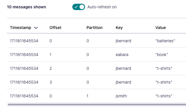
If you go to the terminal, and if you type python3 producer.py getting_started.ini, you should see this as the output:

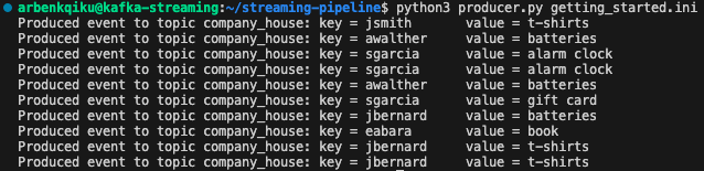
Then, go to the Confluent console, click on Topics and then on your topic name, in my case company_house:

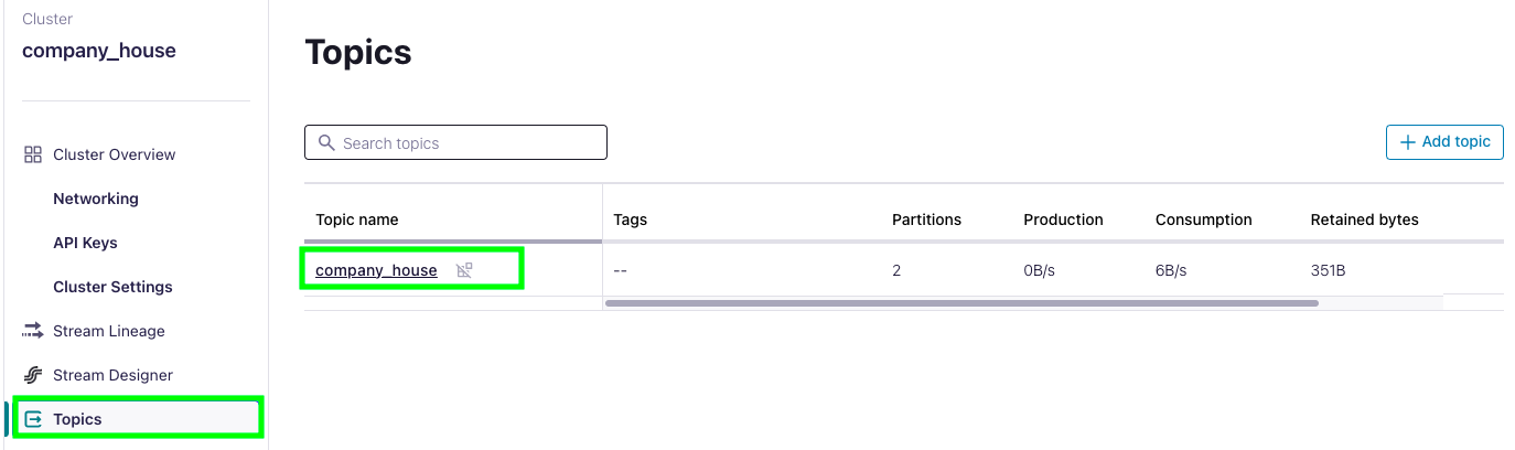
Click on Messages:

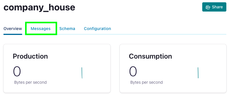
Below, you should see the messages that we just produced to the topic:

This is awesome!

Produce UK’s Companies House Data to a Kafka Topic

So far, we were able to do 2 things:

• Stream data continuously from UK’s Companies House API
• Produce simulated data to our Kafka topic

Now, to integrate these 2 scripts, we need to stream data from UK’s Companies House API and produce it (send it) to our Kafka topic.

Create a file named producer_company_house.py and paste the following code:

#!/usr/bin/env python

import sys
from random import choice
import json
import requests
from argparse import ArgumentParser, FileType
from configparser import ConfigParser
from confluent_kafka import Producer

if __name__ == '__main__':

    url = "https://stream.companieshouse.gov.uk/"

    # Parse the command line.
    parser = ArgumentParser()
    parser.add_argument('config_file', type=FileType('r'))
    args = parser.parse_args()

    # Parse the configuration.
    config_parser = ConfigParser()
    config_parser.read_file(args.config_file)
    config = dict(config_parser['default'])

    # Set idempotence configuration
    config['enable.idempotence'] = 'true'

    # Create Producer instance
    producer = Producer(config)

    try:
        response=requests.get(
            url=url+"companies",
            headers={
                "Authorization": 'Basic ZTA1YjQzYmYtNDY4OC00YWFjLWIxZWItOTY2MWUxYzZjMDA0Og==',
                "Accept": "application/json",
                "Accept-Encoding": "gzip, deflate"
            },
            stream=True
        )

        print("Established connection to Company House UK streaming API")

        for line in response.iter_lines():
            if line:
                decoded_line = line.decode('utf-8')

                json_line = json.loads(decoded_line)

                # Build empty JSON
                company_profile = {
                    "company_name": None,
                    "company_number": None,
                    "company_status": None,
                    "date_of_creation": None,
                    "postal_code": None,
                    "published_at": None
                }

                try:
                    company_profile['company_name'] = json_line["data"]["company_name"]
                except KeyError:
                    company_profile['company_name'] = "NA"

                try:
                    company_profile['company_number'] = json_line["data"]["company_number"]
                except KeyError:
                    company_profile['company_number'] = "NA"
                
                try:
                    company_profile['company_status'] = json_line["data"]["company_status"]
                except KeyError:
                    company_profile['company_status'] = "NA"

                try:
                    company_profile["date_of_creation"] = json_line["data"]["date_of_creation"]
                except KeyError:
                    company_profile["date_of_creation"] = "NA"

                try:
                    company_profile["postal_code"] = json_line["data"]["registered_office_address"]["postal_code"]
                except KeyError:
                    company_profile["postal_code"] = "NA"

                try:
                    company_profile["published_at"] = json_line["event"]["published_at"]
                except KeyError:
                    company_profile["published_at"] = "NA"

                # Produce data to Kafka topics
                topics = {
                    "company_house": company_profile,
                }

                # Optional per-message delivery callback
                def delivery_callback(err, msg):
                    if err:
                        print('ERROR: Message failed delivery: {}'.format(err))
                    else:
                        print("Produced event to topic {}: key = {} value = {}".format(
                            msg.topic(), msg.key(), msg.value()))

                # Produce data to Kafka topics
                for topic, message in topics.items():
                    producer.produce(topic, key=message["company_number"].encode('utf-8'), value=json.dumps(message).encode('utf-8'), callback=delivery_callback)

                # Block until the messages are sent.

    except Exception as e:
        print(f"an error occurred {e}")

Let’s go through the major changes. Here, we define the topic and the content of a specific message with company_profile.

# Produce data to Kafka topics
topics = {
    "company_house": company_profile,
}

Here is what the following code does. It iterates through each topic and message pair in the topics dictionary, extracts the company_number from the message, encodes the company_number and the JSON-formatted message content to UTF-8 encoding using .encode(‘utf-8’) and produces the encoded key-value pair to the Kafka topic using producer.produce().

# Produce data to Kafka topics
for topic, message in topics.items():
    producer.produce(topic, key=message["company_number"].encode('utf-8'), value=json.dumps(message).encode('utf-8'), callback=delivery_callback)

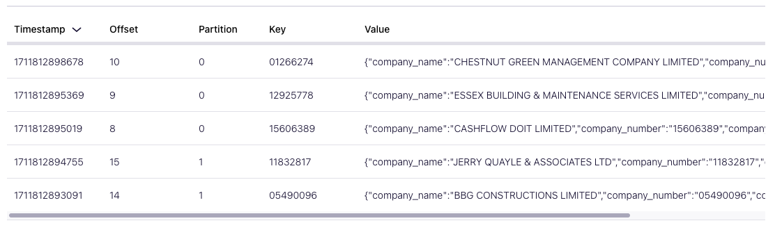
If you type the following code in your terminal python3 producer_company_house.py getting_started.ini, it should stream data from UK’s Companies House and produce it to the Kafka topic company_house. If you go on the Confluent console, you should see incoming messages:

As a next step, we’ll containerize our application.

Containerize our Application

Create a Docker Container of Our Application

A Docker container is a small box that holds everything your application needs to run, like its code, libraries, and settings. This box is like a mini-computer that you can easily move around. Docker containers work similarly. They bundle up all the software and dependencies your application needs into a single package, making it easy to run your application on any computer that has Docker installed. This is very useful because regardless of where you run your container, it will always run consistently. On the other hand, if you share your code with someone else, maybe they don’t have the necessary dependencies to run your code.

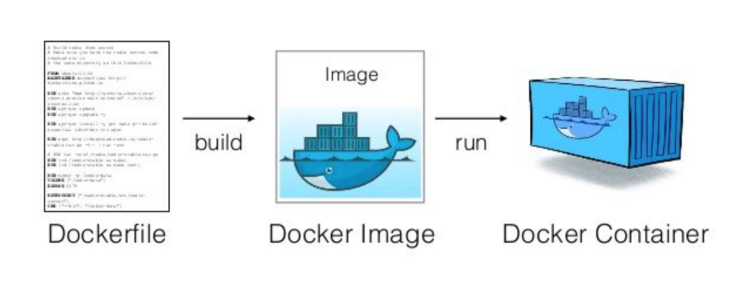
To create a Docker container, you need a Docker image, and to create a Docker image, you need a Dockerfile. A Dockerfile is like a recipe, that shows all the ingredients and steps necessary to prepare a meal. A Docker image is analogous to having the necessary ingredients and appliances ready to cook the meal. It’s a snapshot of a filesystem and its configuration that forms the basis of a container. A Docker container is like the actual prepared meal. It’s a running instance of a Docker image, containing everything needed to run the application, including the code, runtime, libraries, and dependencies.

So, this is what our Dockerfile looks like. Create a new file named Dockerfile and paste the following content. Docker automatically recognizes the file named Dockerfile:

# Use an official Python runtime as a parent image
FROM python:3.10

# Set the working directory in the container
WORKDIR /app

# Copy the current directory contents into the container at /app
COPY . /app

# Install any needed packages specified in requirements.txt
RUN pip install --no-cache-dir -r requirements_docker.txt

# Make the script executable
RUN chmod +x producer_company_house.py

# Run the script with the provided configuration file as an argument
CMD ["./producer_company_house.py", "getting_started.ini"]

Here is what each line of code does. In the following snippet, we are basically taking an existing Docker image and building on top of it. It would be like buying the pre-made dough and then add your toppings to prepare your pizza.

# Use an official Python runtime as a parent image
FROM python:3.10

Here, we are setting the working directory in the container. It is like running cd from the command-line.

# Set the working directory in the container
WORKDIR /app

Here, we are copying the entire content of the current directory, the directory where your Docker image will be created, and paste all the contents.

# Copy the current directory contents into the container at /app
COPY . /app

Here, we install the necessary python packages.

# Install any needed packages specified in requirements.txt
RUN pip install --no-cache-dir -r requirements_docker.txt

Please, create a file named requirements_docker.txt and paste the following content. We are doing this because to produce data to our Kafka topic we don’t need all the packages contained in the file requirements.txt.

configparser==6.0.1
confluent-kafka==2.3.0
requests==2.31.0

This line makes the file producer_company_house.py executable. Making a file executable is necessary to allow it to be run as a program or script. When a file is marked as executable, it means that the operating system recognizes it as a program or script that can be executed directly. Without executable permissions, attempting to run the file will result in a permission denied error.

# Make the script executable
RUN chmod +x producer_company_house.py

Finally, we run the script producer_company_house.py with the config file getting_started.ini as a command-line argument.

# Run the script with the provided configuration file as an argument
CMD ["./producer_company_house.py", "getting_started.ini"]

To create our Docker image from our Dockerfile, we first need to install Docker. Let’s download a GitHub repo that contains the installation for Docker:

git clone https://github.com/MichaelShoemaker/DockerComposeInstall.git

Let’s access the folder that contains the Docker installation:

cd DockerComposeInstall

Let’s modify the file to make it executable:

chmod +x InstallDocker

Then, let’s run it:

./InstallDocker

Type this to verify that Docker has been installed correctly:

docker run hello-world

This should show the following message:

Before proceeding, make sure you saved all the files mentioned in the Dockerfile. If you made any modifications to a file without saving it, the modifications will not be included in the Dockerfile.

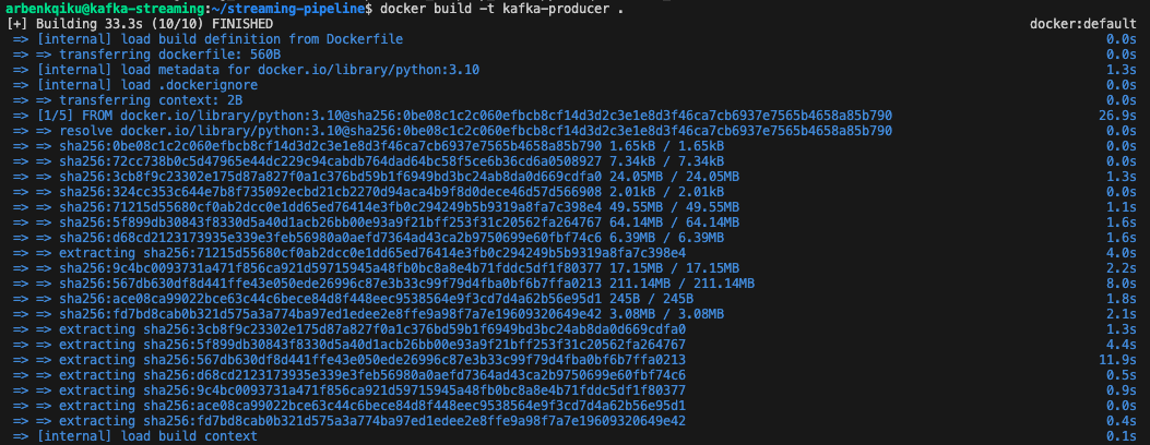
Now, go back to the folder that contains your Dockerfile and type the following. This basically instructs the system to build a docker image called kafka producer from our Dockerfile. The dot at then end indicates the Dockerfile.

docker build -t kafka-producer .

This should build your Docker image:

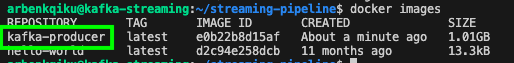
If you type docker images, you should see the Docker image we just built:

To run a container instance of the Docker image, type:

docker run kafka-producer

Now, if you go to Confluent, you’ll see that we’re actually producing data to the company_house topic:

If you go under messages, you should see new incoming messages:

Here are a couple of nifty tricks related to Docker. To see the Docker containers that are currently running, type:

docker ps

To see all Docker containers, type:

docker ps -a

To stop a running Docker container, type:

docker stop container_id

For example:

docker stop a2cd18c97c49

To see restart a Docker container, you don’t need to type docker run image_name again, otherwise you would be running a new instance of the Docker image. Once the Docker container has been created, you can simply restart it:

docker start container_id

To remove a Docker container, first, you need to stop it, then type:

docker rm container_id

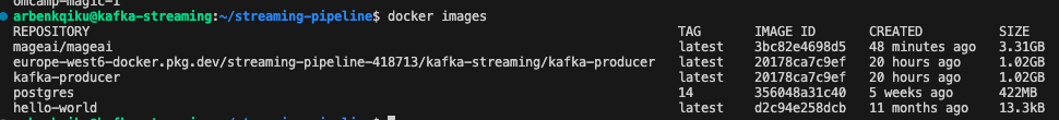
To see all Docker images available, type:

docker images

Now that we know that we can produce data to Kafka, you can stop your Docker container.

So far, we’ve developed a Kafka producer that streams data from the UK’s Companies House API to a Kafka topic. Everything is nicely packaged into a Docker image, from which we’ve launched a Docker container. I would say that this is quite an achievement, congrats!

Up until now, we produced data to a Kafka topic. Right now, we need to consume this data!

From Kafka to BigQuery through Mage

Install Mage

A data orchestrator allows to build ETL (extract, transform and load) data pipelines. That means extracting data from one or multiple systems, apply some transformations to it, and then export it to another system, such as a data warehouse. Mage is a modern and very user-friendly orchestrator, that provides a visually appealing structure of your pipelines:

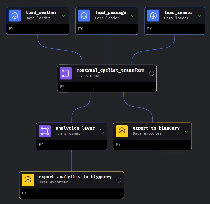
Also, with simple drag and drop you can change how the various blocks interact with each other.

Here is the repo for the installation guide, but we’ll go through the installation here as well.

You can start by cloning the repo:

git clone https://github.com/mage-ai/mage-zoomcamp.git mage-zoomcamp

Navigate to the repo:

cd mage-zoomcamp

Rename dev.env to simply .env — this will ensure the file is not committed to Git by accident, since it will contain credentials in the future.

Now, let’s build the container with Docker compose. When we use Docker Compose to build containers, we’re essentially creating applications made up of multiple containers that can communicate with each other. This is particularly handy for complex applications where different parts of the system need to work together.

In contrast, the usual process of building Docker images involves focusing on creating one container at a time. Each Dockerfile represents a single container, and while these containers can interact, managing their communication and dependencies can become more complex as the application grows.

With Docker Compose, all the details about the containers, such as Docker images, environment variables, and dependencies, are stored in a YAML file. This file acts as a configuration blueprint for our application. For example, in our scenario, we have a YAML file that specifies both a Docker image to install Mage and a PostgreSQL database. Even if we only need Mage for our task, we can still use this YAML file to set up our environment.

docker compose build

Finally, start the Docker container:

docker compose up

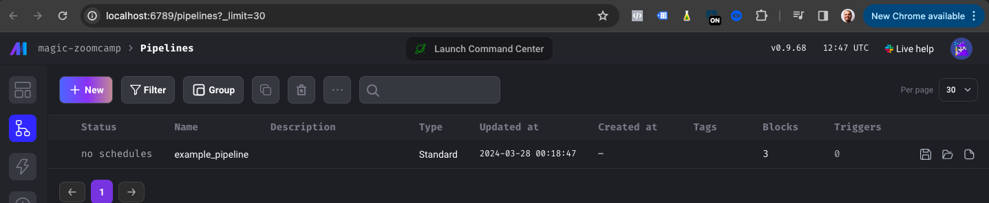
In the YAML file, we have defined Mage’s port as 6789. In fact, you can access Mage by going to your VM and clicking on the browser icon next to port 6789:

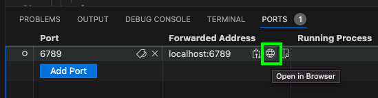
If everything worked correctly, you should be able to access Mage:

However, right now we’re accessing Mage from the our localhost. It would be great to access it via our external IP address.

The external IP address allows users outside the VM’s network to interact with Mage. This can be useful for remote access, enabling team members or clients to use Mage without needing direct access to the VM.

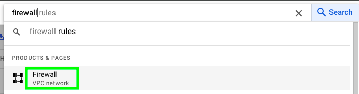
Type firewall in the search bar and click on Firewall:

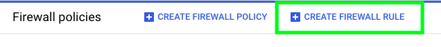
At the top, click on CREATE FIREWALL RULE:

Give a name to your firewall rule, then select the following options and click on CREATE:

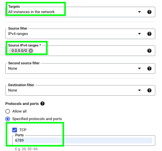
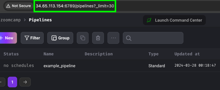
With this, we’re basically allowing ingress traffic through port 6789, which is where Mage is located. Now, go back to your VM, copy your external IP address and type it followed by :6789. This is what it looks like in my case:

34.65.113.154:6789

Now, if you type this address in your browser you should be able to access Mage via the external IP address:

Consume Data from Kafka Topic

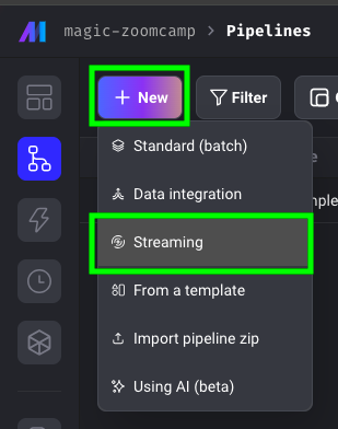
In Mage, you can create either batch or streaming pipelines. In our case, we need to consume data in real-time from a Kafka topic, so we’ll create a streaming pipeline. At the top left, click on New and then on Streaming:

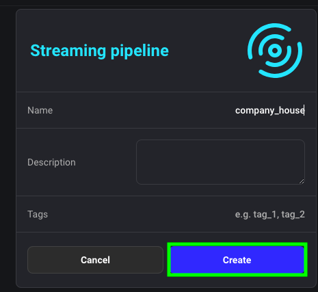
Give a name to your streaming pipeline and click on Create:

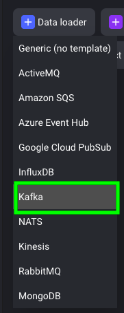
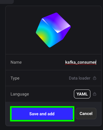
In Mage, a pipeline is composed of blocks. The different blocks are Data loader, Transformer and Data exporter. Your pipeline can have as many blocks as you want. As we need to consume the data from a Kafka topic, click on Data loader and select Kafka:

Give a name to your block and click on Save and add:

Similar to what we did in the file getting_started.ini, we need to define the configuration with the following parameters:

• bootstrap server
• topic
• username
• password

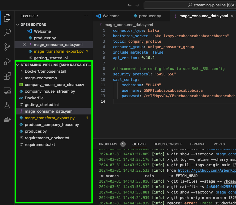
Here is what it should look like:

connector_type: kafka
bootstrap_server: "pkc-lzoyblablablablaluent.cloud:9092"
topic: company_house
consumer_group: unique_consumer_group
include_metadata: false
api_version: 0.10.2

# Uncomment the config below to use SASL_SSL config
security_protocol: "SASL_SSL"
sasl_config:
    mechanism: "PLAIN"
    username: GGPabcabcaabcabca
    password: /rmTFMqsvD4/CEs7tJEZAD6/NV9Oabcabcaabcabcaabcabcaabcabcaabcabca

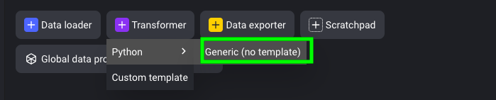
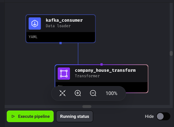
In the Data loader block, we’re consuming the data. However, if you run the pipeline with this block only, there is no output of the consumed data. To see the data, we also need to add a Transformer block. Click on Transformer > Python > Generic (no template):

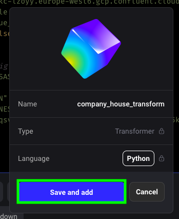
Give a name to your block and click on Save and add:

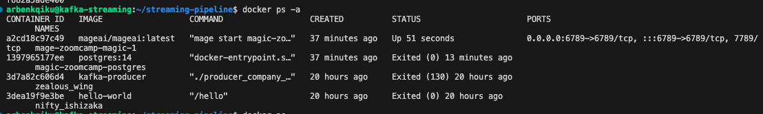
Now, we are ready to consume data. However, we are currently not producing any. To produce data, we can simply start the Docker container that we previously created. So, let’s see what is the container id of our Docker container:

docker ps -a

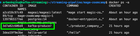
Therefore, we’ll type:

docker start 3d7a82c606d4

Soon enough, on Confluent we should see that we are producing data:

Now, go back to Mage and click on Execute pipeline:

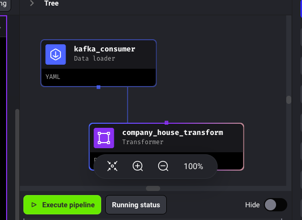
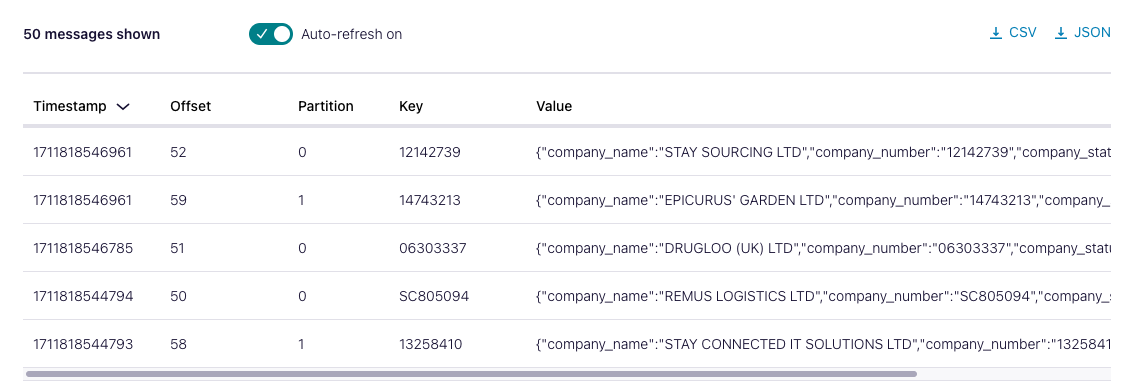
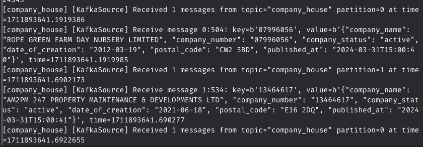
Soon enough, you should see that we’re consuming messages from Kafka:

Congrats! As a next step, we’ll send the streamed data to BigQuery.

Send Streamed Data to BigQuery

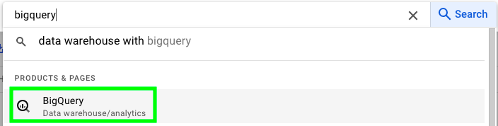
Now, let’s send the data that we’re streaming to BigQuery. To do that, we first need to create a data set in BigQuery. In BigQuery, a data set is the equivalent of a database in other systems. So, go to Google Cloud, type big query and click on BigQuery:

If you havent’ done it already, enable the BigQuery API:

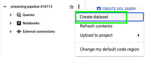
The basic structure of BigQuery is Project > Dataset > Tables. In our case, we first have to create a dataset. Click on the three dots next to your project name and click on Create dataset:

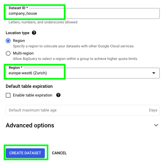
Give a name to your dataset, select a region and click on CREATE DATASET:

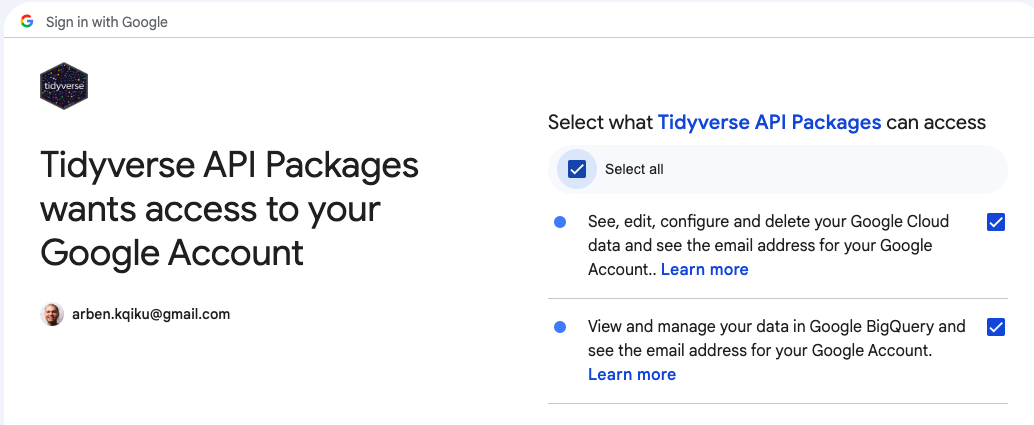
In our case, we’re sending data to BigQuery from Mage, which is a production environement. On the other hand, when you try to send data manually from your local machine, you can login to your Google account through the browser and grant permission to your script to perform tasks. This image provides an example of a manual authentication through the browser to grant access to the Tidyverse API Packages to make changes on BigQuery:

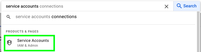
However, in a production environment, we don’t have the luxury to go through the browser’s authentication process, so we need to find another solution to prove to Google that we’re actually authorized to perform tasks. To do that, we can create a service account. A service account is essentially an account authorized to make changes on your behalf. Go to the VM and type service accounts in the search bar and click on Service Accounts:

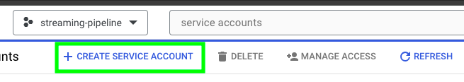
On the top left, click on CREATE SERVICE ACCOUNT:

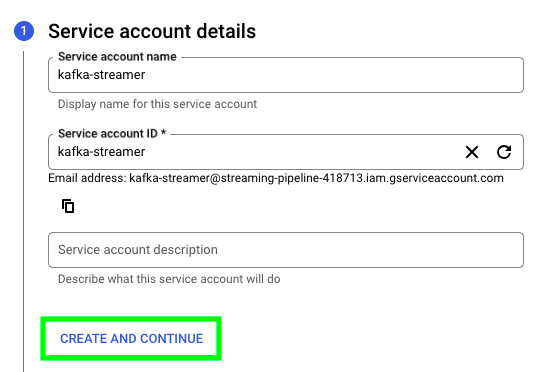
Give a name to your service account and click on CREATE AND CONTINUE:

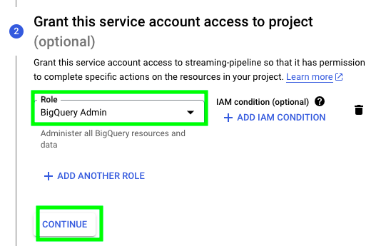
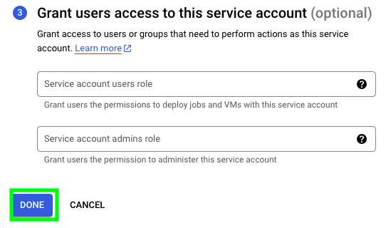
This service account will only interact with BigQuery, so I only gave it BigQuery Admin permissions. If you want your service account to interact with other resources, you should extend your permissions. Click on CONTINUE:

Finally, click on DONE:

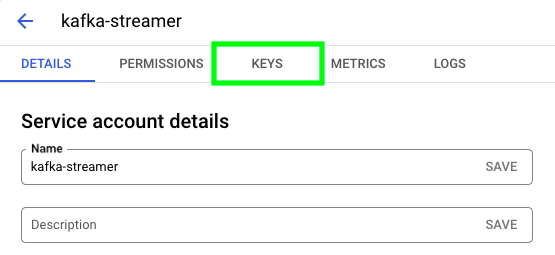
Click on the service account that you just created:

Go to KEYS:

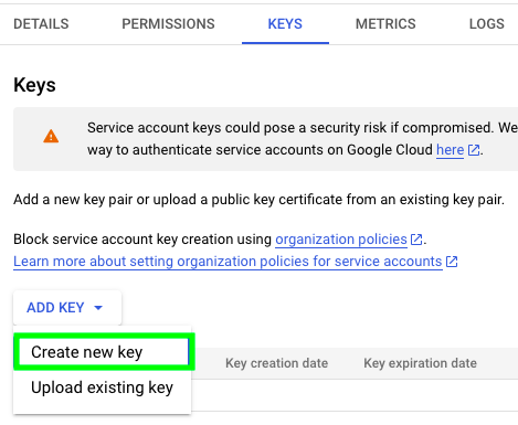
Click on ADD KEY, and then Create new key:

Select JSON and click on CREATE:

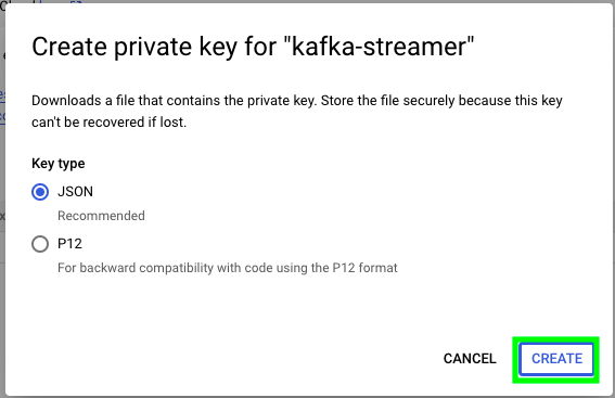
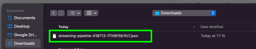
This will download the credentials of the service account that we’ll use to make changes on BigQuery when in a non-interactive environement. To add the credentials to the VM, drag them to this area of VS code:

One of the worst mistakes you could make is to inadvertently publish your credentials to a GitHub repository. To prevent this, we can create a file named .gitignore. Any content listed in this file will be ignored by GitHub, ensuring it’s not published in the current repository. Since our credentials are stored in .json format, to prevent them from being added to our GitHub repository, simply add the following line to your .gitignore file:

# Ignore files with .json extension
*.json

Currently, we’ve only created a dataset in BigQuery. To begin streaming data, we need to create a table. So, let’s start by pushing some mock streaming data to a new table. Open a new python file and paste this code:

import io
import json
import pandas as pd
import pyarrow.parquet as pq
from google.cloud import bigquery # pip install google-cloud-bigquery and pyarrow as a dependency
from google.oauth2 import service_account

credentials = service_account.Credentials.from_service_account_file(
    '/home/arbenkqiku/streaming-pipeline/streaming-pipeline-418713-7f7d915b1fc7.json', scopes=['https://www.googleapis.com/auth/cloud-platform'],
)

client = bigquery.Client(project=credentials.project_id, credentials=credentials)

job_config = bigquery.LoadJobConfig()

json_example = {'company_name': 'CONSULTANCY, PROJECT AND INTERIM MANAGEMENT SERVICES LTD', 'company_number': '13255037', 'company_status': 'active', 'date_of_creation': '2021-03-09', 'postal_code': 'PE6 0RP', 'published_at': '2024-03-23T18:37:03'}
df = pd.DataFrame([json_example])

df['date_of_creation'] = pd.to_datetime(df['date_of_creation'])
df['published_at'] = pd.to_datetime(df['published_at'])

table_name = 'company_house_stream'

table_id = '{0}.{1}.{2}'.format(credentials.project_id, "company_house", table_name)
job_config.write_disposition = bigquery.WriteDisposition.WRITE_APPEND

# Upload new set incrementally:
# ! This method requires pyarrow to be installed:
job = client.load_table_from_dataframe(
    df, table_id, job_config=job_config
)

Let’s analyze what this code snippet does. The first piece of code loads service account credentials from a JSON key file located at /home/arbenkqiku/streaming-pipeline/streaming-pipeline-418713-7f7d915b1fc7.json. These credentials are used to authenticate with Google Cloud services, in our case with BigQuery.

credentials = service_account.Credentials.from_service_account_file(
    '/home/arbenkqiku/streaming-pipeline/streaming-pipeline-418713-7f7d915b1fc7.json', scopes=['https://www.googleapis.com/auth/cloud-platform'],
)

The next code snippet initializes a BigQuery client using the obtained credentials and specifies the project ID associated with those credentials and creates a BigQuery load job configuration (job_config):

client = bigquery.Client(project=credentials.project_id, credentials=credentials)
job_config = bigquery.LoadJobConfig()

The following code snippet creates a DataFrame df containing a single example record json_example representing data to be loaded into BigQuery. This record includes fields like ‘company_name’, ‘company_number’, ‘company_status’, etc. It then converts date fields (‘date_of_creation’ and ‘published_at’) in the DataFrame to datetime objects using pd.to_datetime() to ensure compatibility with BigQuery’s date format.

json_example = {'company_name': 'CONSULTANCY, PROJECT AND INTERIM MANAGEMENT SERVICES LTD', 'company_number': '13255037', 'company_status': 'active', 'date_of_creation': '2021-03-09', 'postal_code': 'PE6 0RP', 'published_at': '2024-03-23T18:37:03'}
df = pd.DataFrame([json_example])

df['date_of_creation'] = pd.to_datetime(df['date_of_creation'])
df['published_at'] = pd.to_datetime(df['published_at'])

Here we define the destination table_id where the DataFrame data will be loaded. This table is located in the company_house dataset within the specified project.

table_name = 'company_house_stream'
table_id = '{0}.{1}.{2}'.format(credentials.project_id, "company_house", table_name)

This configures the job to append the DataFrame data to the existing table if it already exists.

job_config.write_disposition = bigquery.WriteDisposition.WRITE_APPEND

Finally, this initiates a BigQuery load job job to upload the DataFrame data to the specified table.

# Upload new set incrementally:
# ! This method requires pyarrow to be installed:
job = client.load_table_from_dataframe(
    df, table_id, job_config=job_config
)

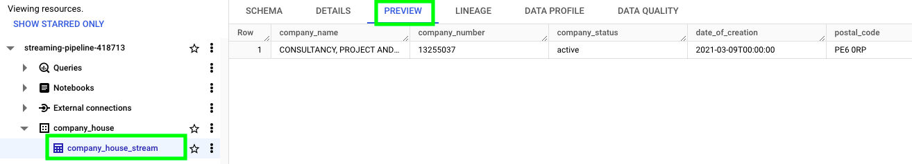
If you now go to BigQuery, you should see a table named company_house_stream. If you click on PREVIEW, you should see the mock-up data that we sent.

Now, let’s got back on Mage to the transfomer block, remove the existing code and add this code:

from typing import Dict, List
import pandas as pd
import pyarrow as pa
from google.cloud import bigquery
from google.oauth2 import service_account

if 'transformer' not in globals():
    from mage_ai.data_preparation.decorators import transformer

@transformer
def transform(messages: List[Dict], *args, **kwargs):

    # define container for incoming messages
    incoming_messages = []

    counter = 1
    for msg in messages:
        # print(counter)
        counter += 1
        # print(msg)

        # append each message
        incoming_messages.append(msg)
    
    # turn into a pandas data frame
    df = pd.DataFrame(incoming_messages)

    # convert string columns to date or date time
    df['date_of_creation'] = pd.to_datetime(df['date_of_creation'])
    df['published_at'] = pd.to_datetime(df['published_at'])

    # define credentials
    credentials = service_account.Credentials.from_service_account_file(
        '/home/src/streaming-pipeline-418713-7f7d915b1fc7.json', scopes=['https://www.googleapis.com/auth/cloud-platform'],
    )

    # define client
    client = bigquery.Client(project=credentials.project_id, credentials=credentials)

    # define job
    job_config = bigquery.LoadJobConfig()

    # define table name and big query details
    table_name = 'company_house_stream'
    table_id = '{0}.{1}.{2}'.format(credentials.project_id, "company_house", table_name)
    job_config.write_disposition = bigquery.WriteDisposition.WRITE_APPEND

    print("BLOCK 3.1")

    print(df)

    # Upload new set incrementally:
    # ! This method requires pyarrow to be installed:
    job = client.load_table_from_dataframe(
        df, table_id, job_config=job_config
    )

    print(df.head())

    return df

Let’s analyze this code. Here we iterate over each message in the messages list and append it to a new list called incoming_messages. This is essentially collecting all the incoming messages from Kafka into a single list.

# define container for incoming messages
incoming_messages = []

counter = 1
for msg in messages:
    # print(counter)
    counter += 1
    # print(msg)

    # append each message
    incoming_messages.append(msg)

This converts the list of dictionaries incoming_messages into a Pandas DataFrame df.

    # turn into a pandas data frame
    df = pd.DataFrame(incoming_messages)

The rest of the code is basically the same as the previous script. The only thing that really changes is the location of our credentials, as we’re now in Mage and not in the VM:

# define credentials
credentials = service_account.Credentials.from_service_account_file(
    '/home/src/streaming-pipeline-418713-7f7d915b1fc7.json', scopes=['https://www.googleapis.com/auth/cloud-platform'],
)

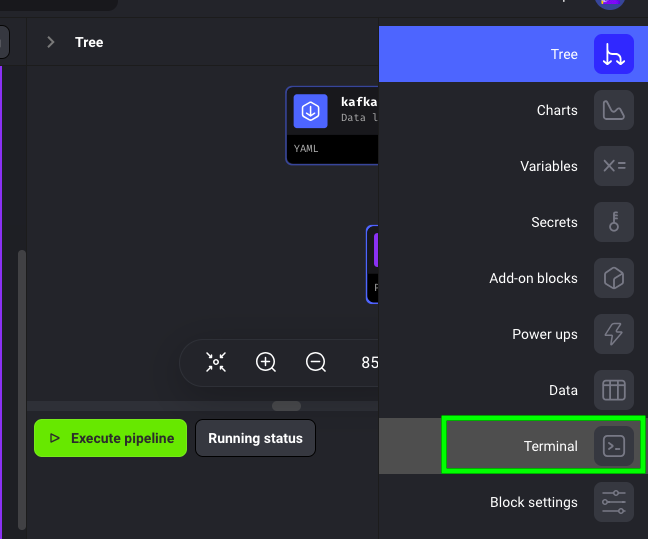
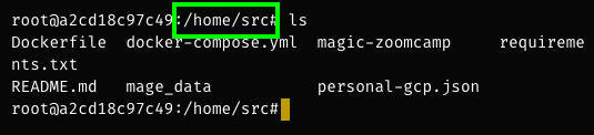
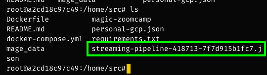
One of the cool features of Mage is that you can access its internal terminal, and see what files are available and what are the respective paths:

First of all, as you can see the default path in Mage starts with /home/src. However, when we type ls the credentials are nowhere to be seen:

This is because we actually need to drag our credentials into the Mage folder:

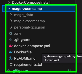
Once we do that, we see that the credentials are available:

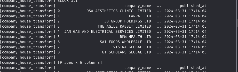
Now we are able to test the pipeline! Go back to the terminal and start the Docker container that produces data to the Kafka topic. Once you see incoming data on Confluent, go to Mage and click on Execute pipeline:

On Mage, you should see the data that we’re consuming:

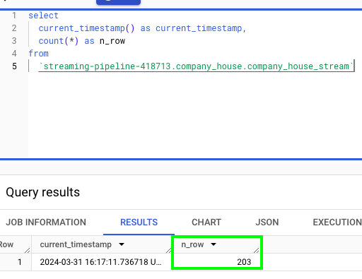
On BigQuery, you should see the number of rows gradually increasing:

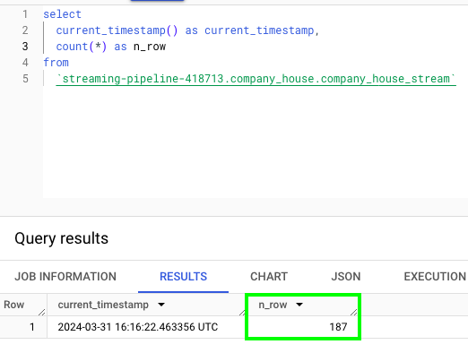
Here is approximately 1 minute later:

Congrats! We just built a working streaming pipeline, that:

• Streams data from UK’s Companies House API
• Produces it to a Kafka topic
• Consumes it from a Kafka topic
• And finally streams it to a BigQuery table

Create Table that Contains all UK’s Companies House Data

For now, let’s stop our Docker container that produces data to the Kafka topic and cancel our pipeline on Mage. Next, we need to create a BigQuery table containing all the available data from the UK’s Companies House up to March 2024. I downloaded the data from here and cleaned it up. You can find the cleaned data here; please download it. In the next step, as we stream incoming data, we’ll merge it with this table containg all the available data.

Here is the script to send the overall table of UK’s Companies House data to BigQuery. Given the size of the table, namely 437 MB, I was not able to run the script in my VM so I had to run it locally, which took almost 15 minutes. Anyway, this does not have any incidence on our project as in the end everything will run programmatically in the cloud.

import io
import json
import pandas as pd
import pyarrow.parquet as pq
from google.cloud import bigquery # pip install google-cloud-bigquery and pyarrow as a dependency
from google.oauth2 import service_account

credentials = service_account.Credentials.from_service_account_file(
    '/home/arbenkqiku/streaming-pipeline/mage-zoomcamp/streaming-pipeline-418713-7f7d915b1fc7.json', scopes=['https://www.googleapis.com/auth/cloud-platform'],
)

df = pd.read_csv("company_house_core_clean.csv")

client = bigquery.Client(project=credentials.project_id, credentials=credentials)

job_config = bigquery.LoadJobConfig()

table_name = 'company_house_core'

table_id = '{0}.{1}.{2}'.format(credentials.project_id, "company_house", table_name)
job_config.write_disposition = bigquery.WriteDisposition.WRITE_APPEND

# Upload new set incrementally:
# ! This method requires pyarrow to be installed:
job = client.load_table_from_dataframe(
    df, table_id, job_config=job_config
)

These are the only two aspects that differ from the previous script. First of all, we read a csv of the clean data. Then, the table name changes.

df = pd.read_csv("company_house_core_clean.csv")

table_name = 'company_house_core'

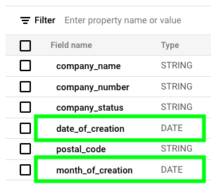
Please makre sure that the columns date_of_creation and month_of_creation are of type DATE:

Apply Transformations with dbt (data build tool)

How to Set-Up dbt

dbt, also known as Data Build Tool, is designed for data transformation tasks. It enables the creation of reusable modules, which are essentially reusable blocks of SQL code that can be consistently applied across different scenarios. For example, you can ensure that a KPI is calculated in a standardized manner by utilizing the same dbt module across various contexts. Additionally, dbt introduces programming language features such as functions and variables into SQL workflows, expanding the capabilities beyond traditional SQL. Furthermore, dbt offers version control, a feature typically absent in SQL environments, allowing for better management and tracking of changes to data transformations.

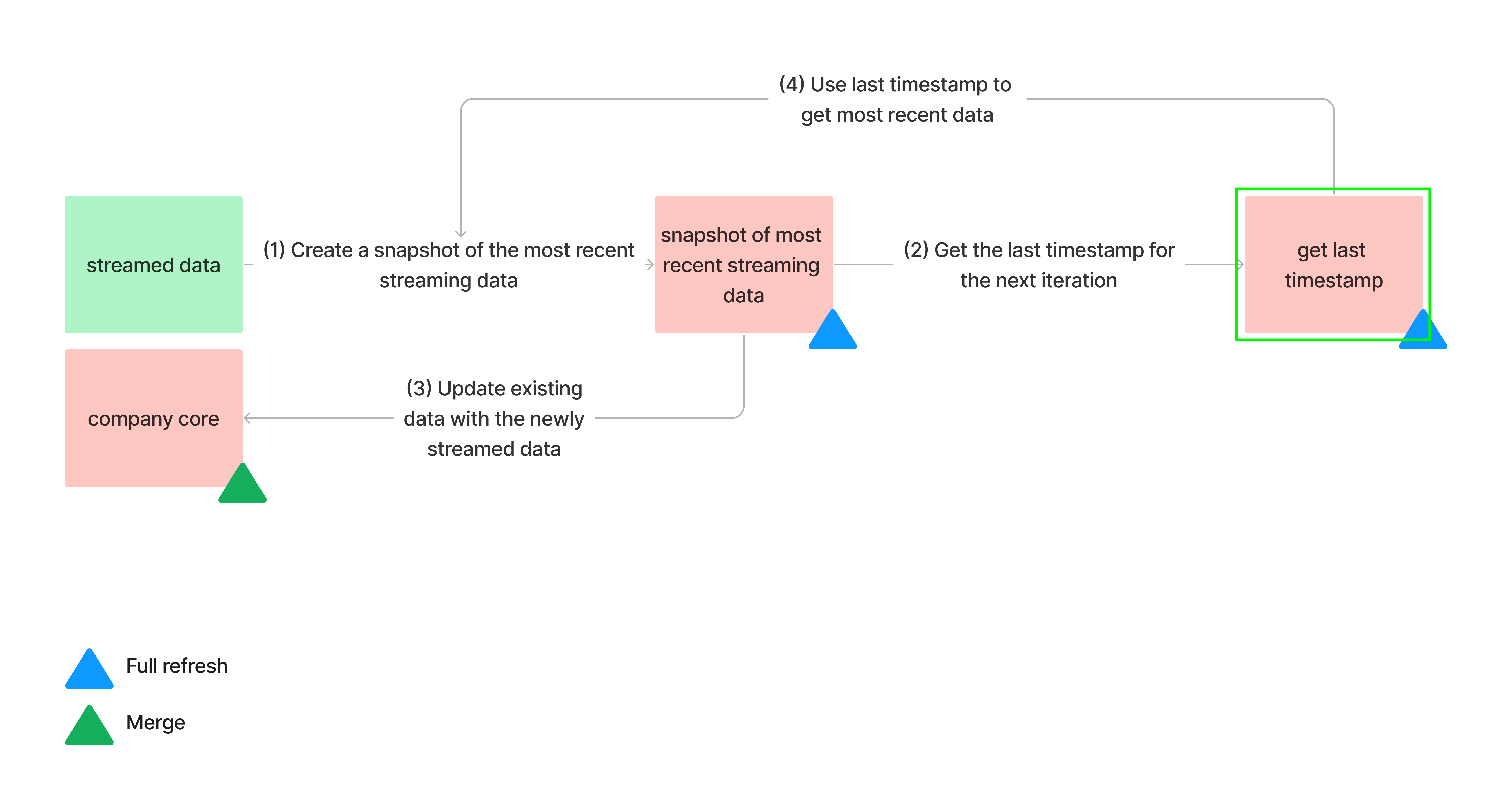
In our case, we’ll use dbt to create the following workflow:

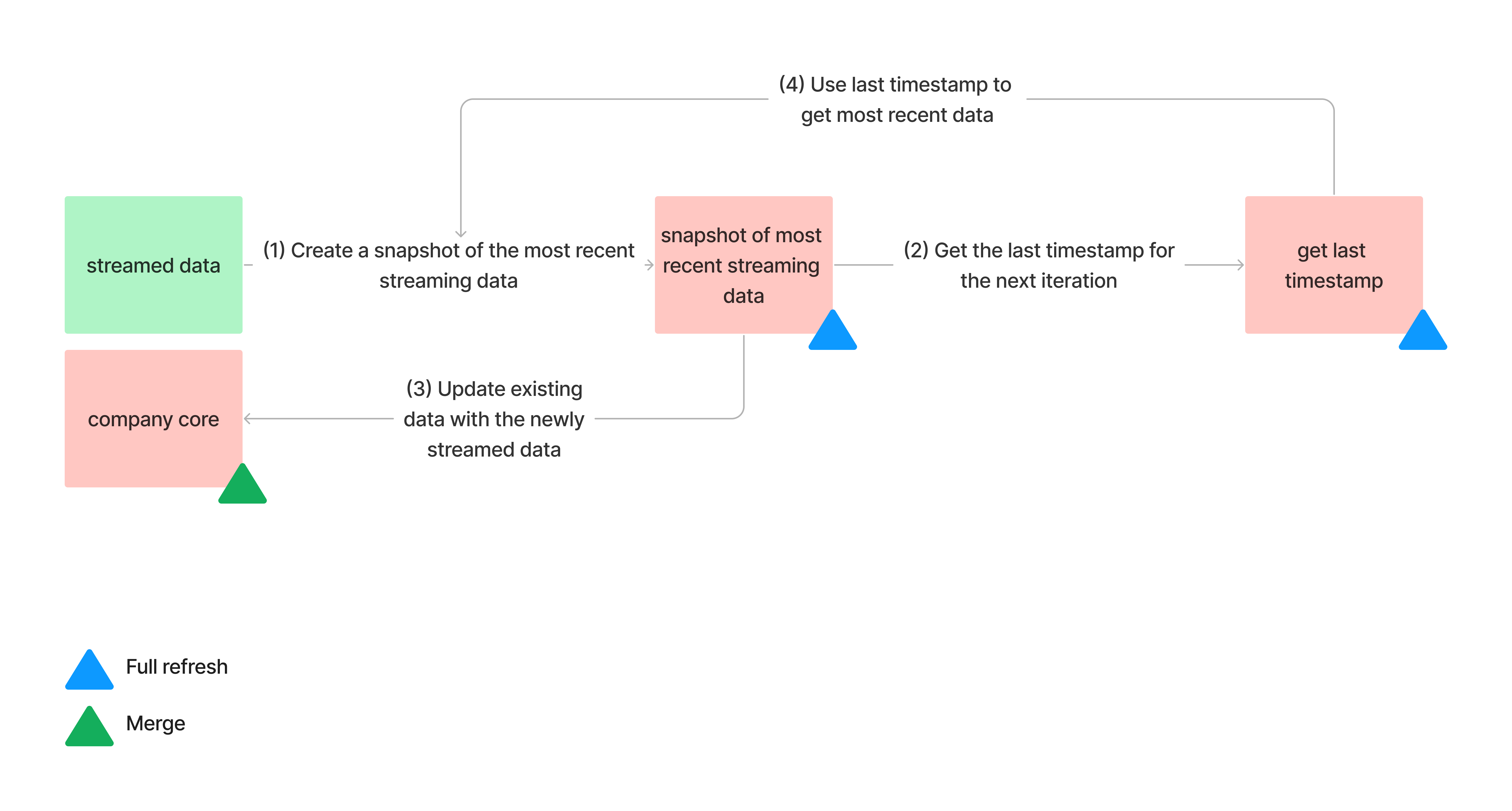
• (1) As new data is streamed in, we capture a snapshot of the latest information, which includes all data accumulated since the previous snapshot was taken.
• (2) From this data, we extract the most recent timestamp available. This timestamp will be helpful for retrieving the next snapshot.
• (3) Subsequently, we utilize the snapshot to update the overall UK’s Companies House data.
• This process repeats as we capture another snapshot of the most recent streamed data, using the last timestamp from the previous snapshot.

This enables continuous updates to the UK’s Companies House data as new data is streamed.

Let’s set up dbt. To start, we’ll focus on two key tasks:

• Linking GitHub Repository with dbt for Versioning: this involves connecting your GitHub repository with dbt to enable version control.
• Linking BigQuery with dbt for Data Retrieval and Pushing: this step entails establishing a connection between BigQuery and dbt, allowing you to retrieve data from BigQuery and push transformed data back into BigQuery.

Go to this link and click on Create a free account:

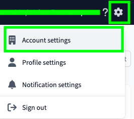
Click on the settings icon on the top right and the click on Account settings:

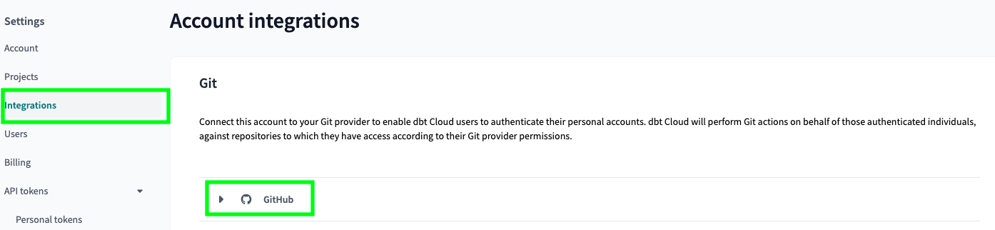
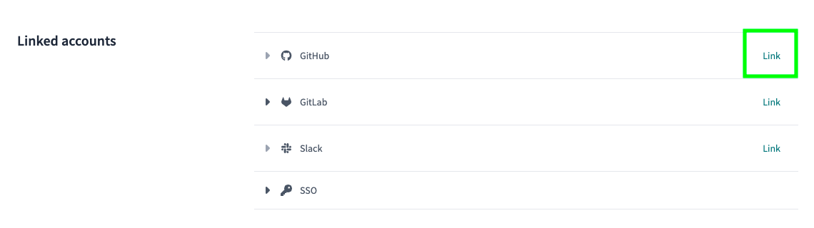
On the left side, click on Integrations and then on GitHub:

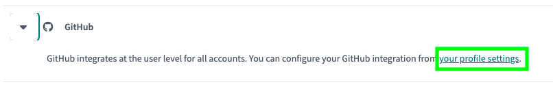
Click on your profile settings:

Click on Link at the GitHub row and follow the process:

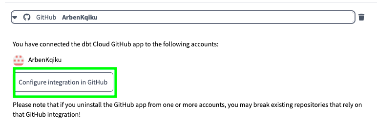
Come back and click on Configure integration in GitHub:

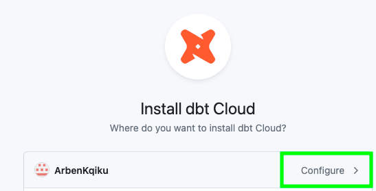
Select your account and click on Configure:

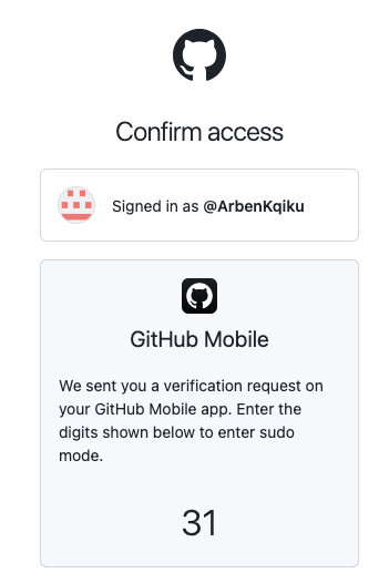
In my case, I am confirming my access through my GitHub app:

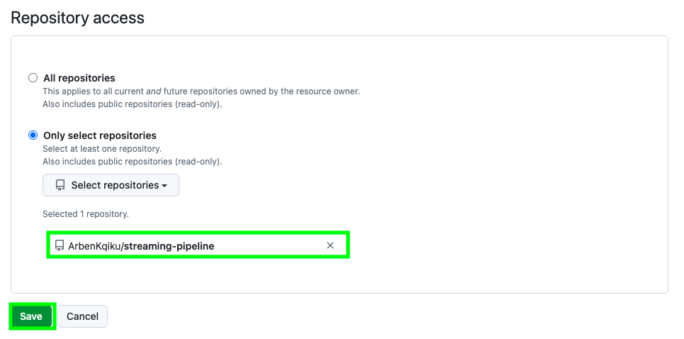
Give it access to your repo and click on Save:

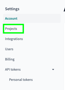
Now, go back to dbt and click on projects:

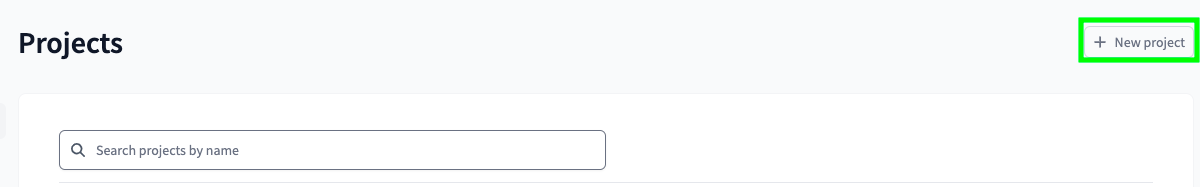
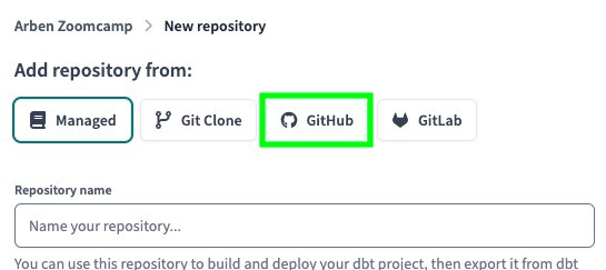
If you don’t have a project click on New project:

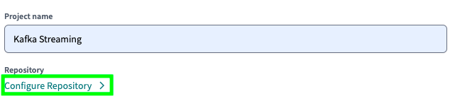
Give a name to your project and click on Configure Repository:

Click on GitHub:

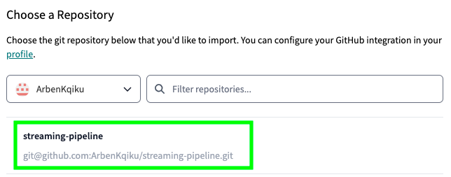
Choose the repo that you just configured:

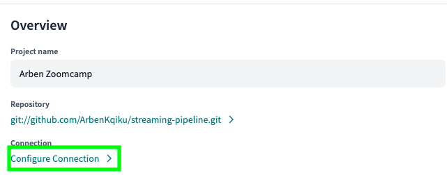
Now, click on Configure Connection:

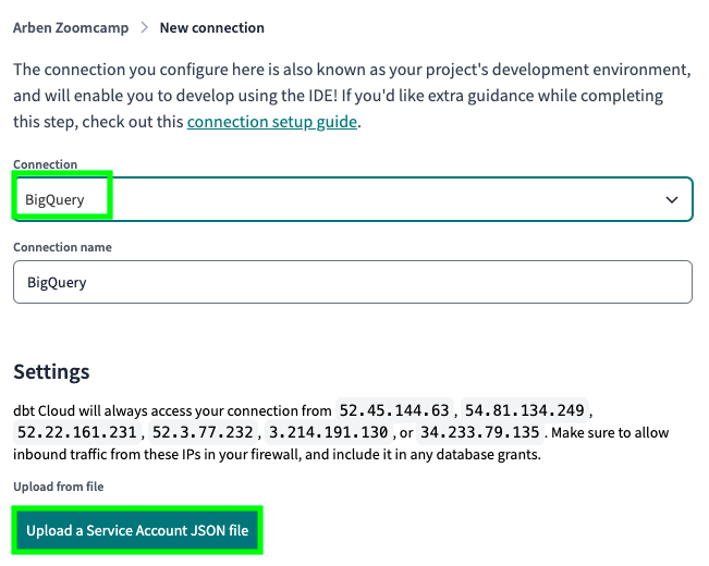
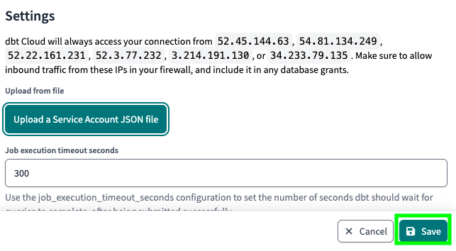
Select BigQuery and click on Upload a Service Account JSON file:

Select the JSON file (the credentials) that we previously created, the same that we used to upload the entire UK’s Companies House data set:

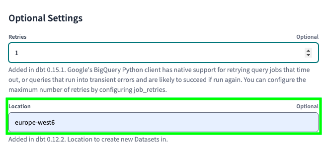
Make sure the location matches the datasets in BigQuery. Otherwise, dbt won’t be able to use the existing tables to create new ones:

Finally, click on Save:

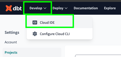
Once you’re done, on the top left, click on Develop and on Cloud IDE:

On the left side, click on Initialize dbt project:

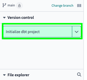
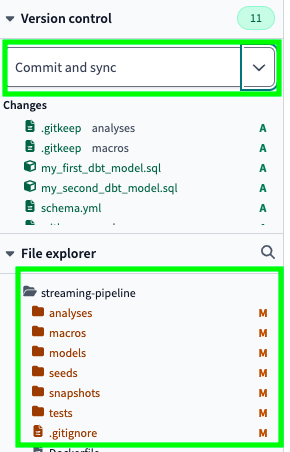
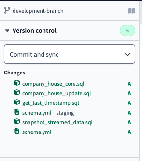
As you can see, some files, which represent the basic structure of a dbt project, were created. Click on Commit and sync to push the changes to the GitHub repository:

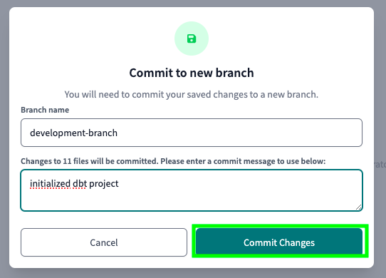
As mentioned earlier, dbt enforces good software development practices. In this case, it is asking us to create a new branch and to commit to it. Give a name to your new branch, add a message to your commit and click on Commit Changes:

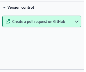
Once your new branch has been created, and you are done with your development, you can click on Create a pull request on GitHub:

Click on Create pull request:

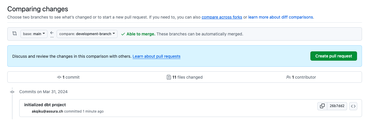
If there are no conflicts, GitHub will tell you that you can merge with the main branch. Click on Merge pull request and then Confirm merge:

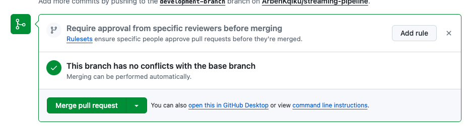
In theory, now you could safely delete your development branch. However, in our case we have just started, so we won’t delete it yet.

Create dbt Data Sources

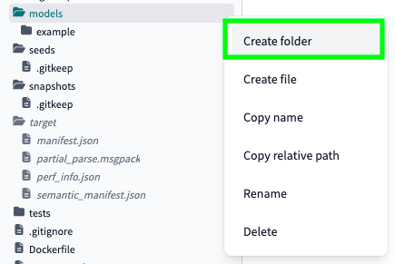
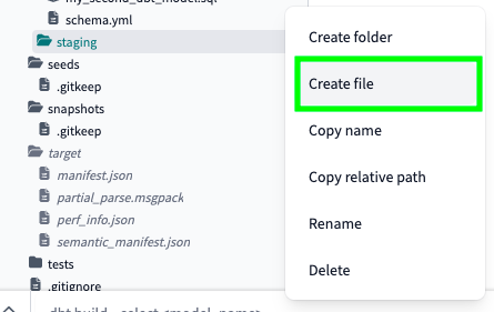
First of all, let’s create a new folder for our staging models and data sources. In fact, to create data models, you need data sources. Click on the three dots next to the models folder, and click on Create folder:

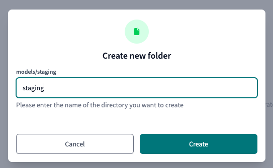
Call your folder staging and click on Create:

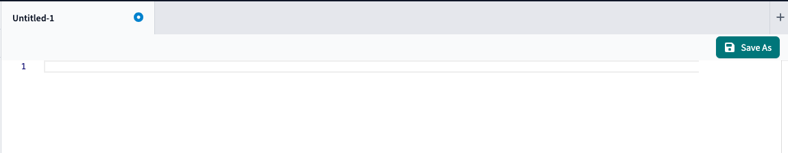
Within the staging folder, click on Create file:

Click on Save as at the top right:

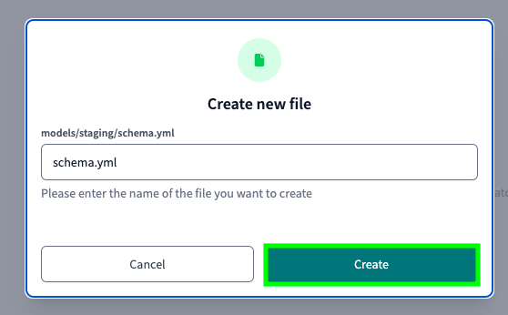
Name your file schema.yml and click on Create:

Paste the following code:

version: 2

sources:
  - name: staging
    database: streaming-pipeline-418713 # BigQuery project id
    schema: company_house # BigQuery data set
    tables:
      - name: company_house_core
      - name: company_house_stream

In this configuration:

• version: 2: Specifies the version of the YAML configuration file.
• sources: Defines the data sources used in the project.
• name: staging: Provides a name for the data source.
• database: streaming-pipeline-418713: Specifies the BigQuery project ID where the data resides.
• schema: company_house: Indicates the BigQuery dataset containing the tables.
• tables: Lists the tables within the specified dataset.
• name: company_house_core: Names one of the tables within the dataset.
• name: company_house_stream: Names another table within the dataset.

This configuration allows dbt to locate and access the specified data in BigQuery. It is essentially a representation of the data that we have in BigQuery:

Create dbt Models

Let’s begin constructing our initial model. We encounter a classic “chicken and egg” scenario: we require a snapshot of the most recent data, yet we lack a timestamp. To address this, our first step is to generate a timestamp.

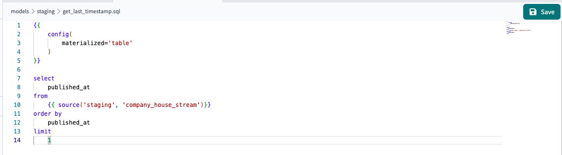
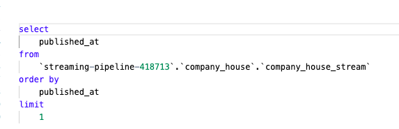
In the staging folder, create a file named get_last_timestamp.sql and paste the following code. This code snippet is written in Jinja templating language. This is used by dbt for managing and transforming data in data warehouses.

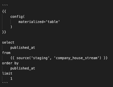
Unfortunately, for some reason my site was not able to parse jinja code, so, I’ll simply paste here an image of the code. In any case, you can find the code in my GitHub repo.

Here’s a breakdown of what each part of the code does:

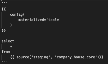
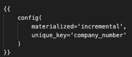
The config part is a Jinja directive used to configure settings for the dbt model. In this case, it sets the materialization method for the dbt model to table, indicating that the results of the SQL query will be stored in a table.

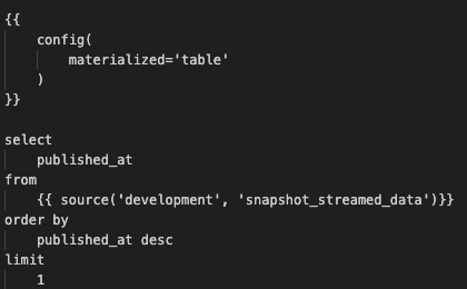
select published_at from order by published_at limit 1: This is a SQL query written inside the Jinja template. It selects the published_at column from the company_house_stream table in the staging schema. The “” syntax is a Jinja function call that dynamically generates the name of the table based on the provided arguments.

In this query, we’re selecting the first timestamp because it represents the initial retrieval of streamed data. However, for subsequent iterations, we’ll use the last timestamp from the previous snapshot, as we want the most recent timestamp.

order by
    published_at desc
limit
    1

Once you have created your model, click on Save at the top right:

At the bottom, if you click on Compile:

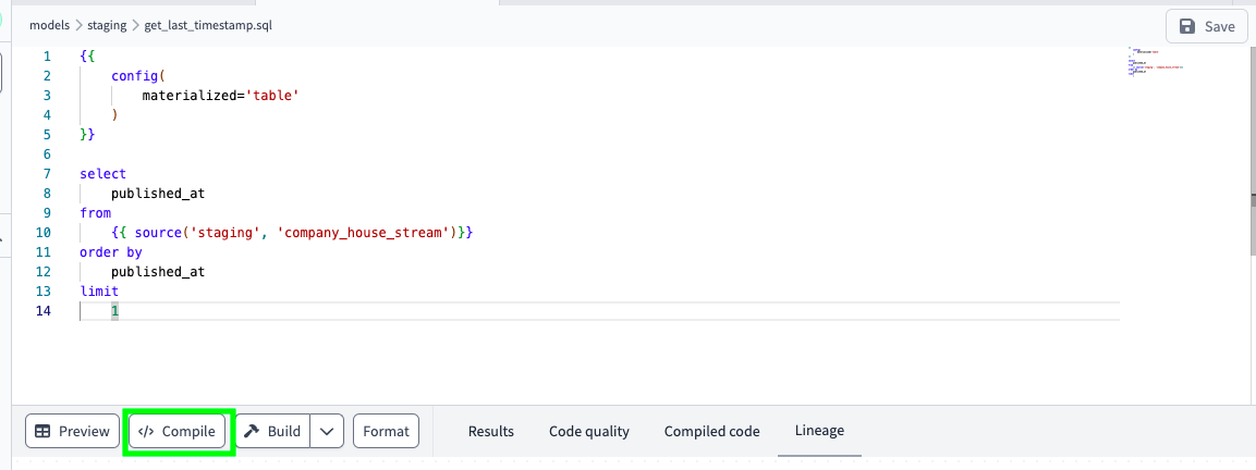
You can see what the code looks like in actual SQL:

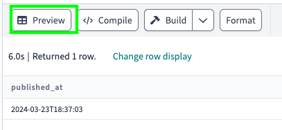
If you click on Preview, you can see what the actual result would be:

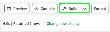
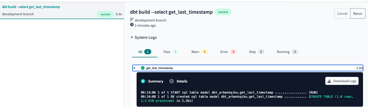
If you click on Build, it would build your model, which means that a table named get_last_timestamp will be created:

If you click at the bottom left corner:

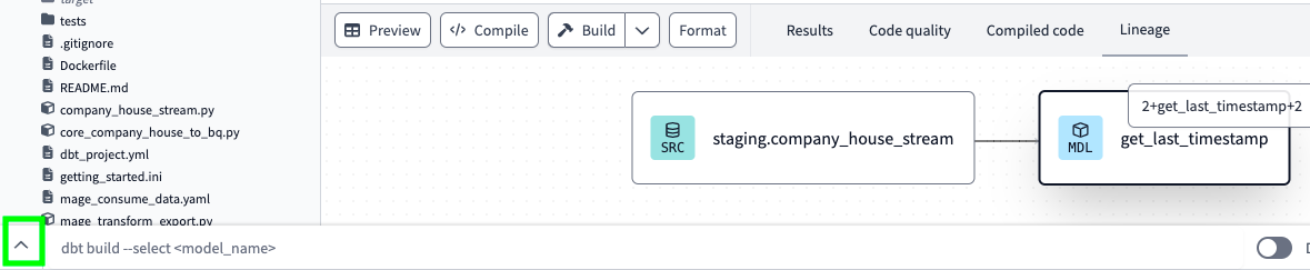
You can see the details that went into building your model:

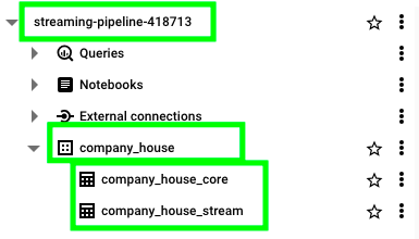
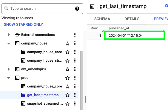
Now, on BigQuery you should see a new dataset called dbt_ followed by your username, in addition to the table get_last_timestamp:

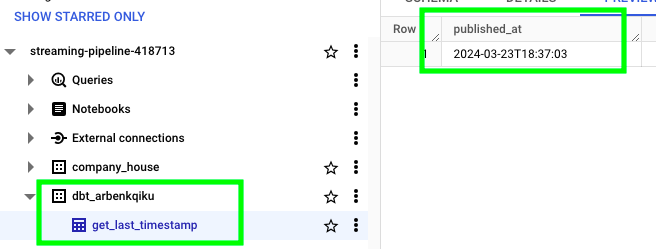
The dataset has this name because we’re still in a development environement. Later, when we’ll push our dbt models to production, a new dataset called prod will be created.

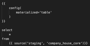
While developing, given that we’ll integrate the newly streamed data into the complete UK’s Companies House data, and given that our models will be pushed to the dbt_arbenkqiku dataset, we need to have the complete UK’s Companies House data in our development dataset as well. Create a new dbt model called company_house_core.sql and paste the following code:

Save the model and click on Build. In BigQuery, next to the development dataset, click on the three dots and then click on Refresh contents:

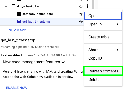
You should see a replica of the complete UK’s Companies House data:

Now that we have a new dataset with two tables, we can add them to our configuration file schema.yml. We can call these sources development:

version: 2

sources:
  - name: staging
    database: streaming-pipeline-418713 # BigQuery project id
    schema: company_house # BigQuery data set
    tables:
      - name: company_house_core
      - name: company_house_stream
  - name: development
    database: streaming-pipeline-418713 # BigQuery project id
    schema: dbt_arbenkqiku # BigQuery data set
    tables:
      - name: company_house_core
      - name: get_last_timestamp

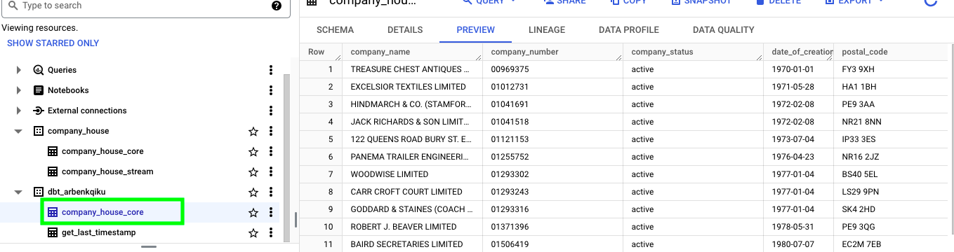
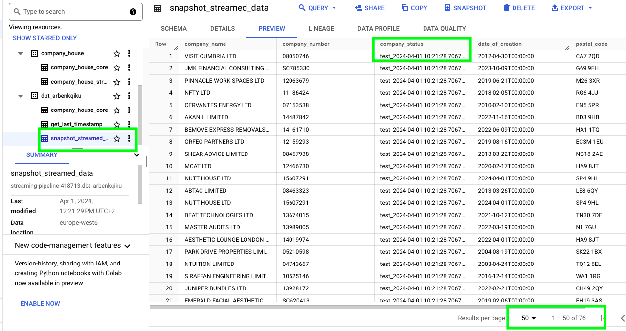
Now, create a new dbt model named snapshot_streamed_data.sql and paste the following code:

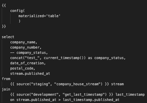
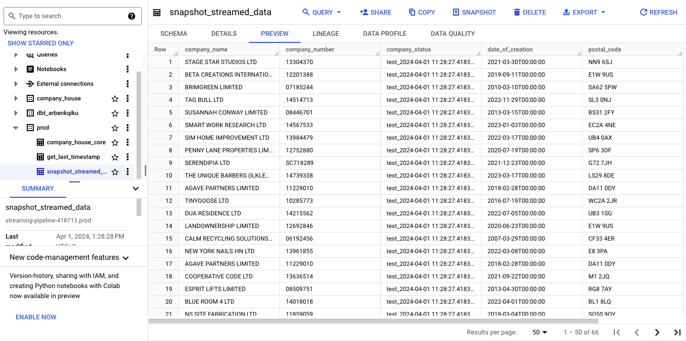
In this code, by using the timestamp that we retrieved earlier, we only get the data that is newer then the last timestamp. This is reflected in the condition stream.published_at > last_timestamp.published_at. This ensures that we create a snapshot of the most recent data. Also, here I purposely modify the company status with concat("test_", current_timestamp()) as company_status. This is because later we will merge the snapshot of the streamed data with the main table, and I want to ensure that the data in the main table is properly updated. Of course, later we’ll use the actual company_status. Save your dbt model and build it.

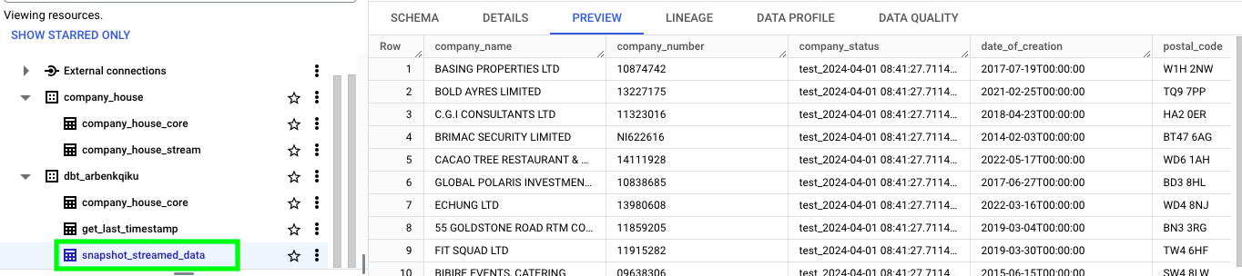
If everything worked correctly, you should see a new table named snapshot_streamed_data:

Also, let’s add this new table to our configuration file by adding this line:

- name: snapshot_streamed_data

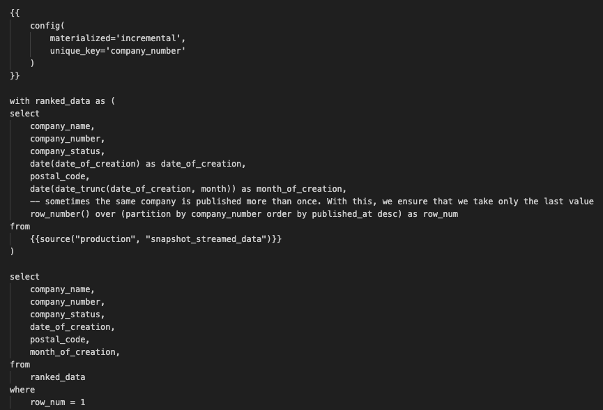
Now, let’s integrate the streamed data in the complete UK’s Companies House data. To do so, we need to replace the content of the dbt model called company_house_core.sql with the following code. This is because we want to update the BigQuery table called company_house_core:

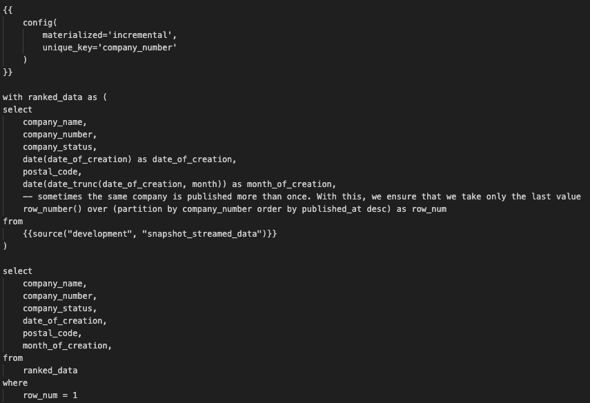
The following code snippet implements an incremental materialization strategy, which means updating the table instead of recreating it. Specifically, it updates rows based on a unique identifier called company_number. The model compares existing data with incoming data for each company_number and updates rows if there are any differences.

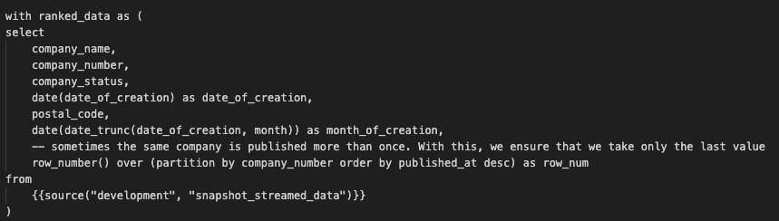
Here we create a common table expression (CTE) named ranked_data. We do this because we want to able to filter out duplicate rows. In this line of code specifically row_number() over (partition by company_number order by published_at desc) as row_num, with this window function we group data by company number, order it by the column published_at in descending order, and count the row numbers.

Finally, with the condition row_num = 1, we only select the most recent instance for each company_number.

select
    company_name,
    company_number,
    company_status,
    date_of_creation,
    postal_code,
    month_of_creation,
from
    ranked_data
where
    row_num = 1

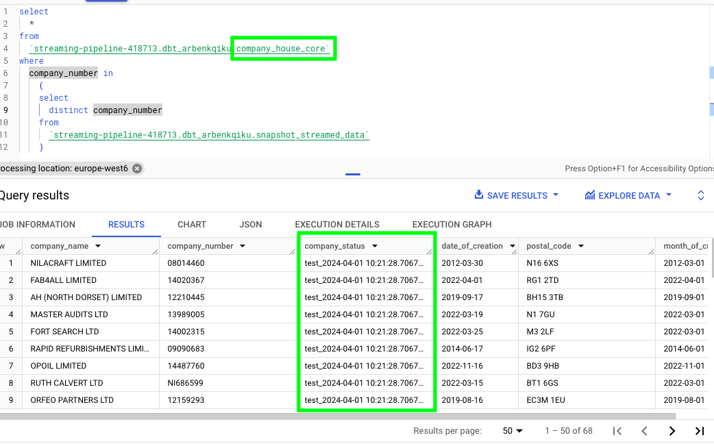
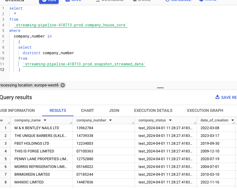
Now, we need to verify that the data has been updated correctly in the company_house_core table. If we run this query in BigQuery, where we’re essentially extracting the rows from the company_house_core table that match a company_number contained in the table snapshot_streamed_data:

select
  *
from
  `streaming-pipeline-418713.dbt_arbenkqiku.company_house_core`
where
  company_number in 
    (
    select
      distinct company_number
    from
      `streaming-pipeline-418713.dbt_arbenkqiku.snapshot_streamed_data`
    )

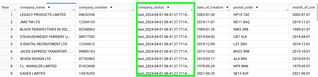
We can see that the column company_status matches the artifically created column:

Test the Entire Pipeline in a Development Environment

First of all, in the dbt model get_last_timestamp.sql, replace order by published_at with order by published_at desc, as we want to get the last timestamp. Also, replace the source as we want to get the last timestamp from the most recent snapshot. This is what the final code looks like:

Save the dbt model and click on Build. Now, if you check the timestamp in the table get_last_timestamp, you should have the most recent timestamp available from the table snapshot_streamed_data:

Now, go to the terminal and start the Docker container that produces data to the Kafka topic. When you see production data in the Confluent console, start the Mage streaming pipeline as well. After a couple of minutes, stop these 2 process as we have generated enough new data to test things in our dbt development environment.

In dbt, build (run) the model snapshot_streamed_data.sql. If you then go to BigQuery, you should see that the table snapshot_streamed_data only contains the most recent streamed data.

Finally, we can build model company_house_core.sql. If we extract the unique company_number values from the company_house_core table, we can see that the data has been updated successfully:

Right now, we are on the development branch of our GitHub repo. To use our dbt models in production, we need to make a pull request to our main branch, and then merge the dev branch with the main branch, as we did at the beginning of the dbt section:

Test the Pipeline in Production

In dbt production, a new dataset named prod will be created. However, the entire UK’s Companies House data does not exist in this dataset. So, in the dbt model company_house_core.sql replace the content with this code:

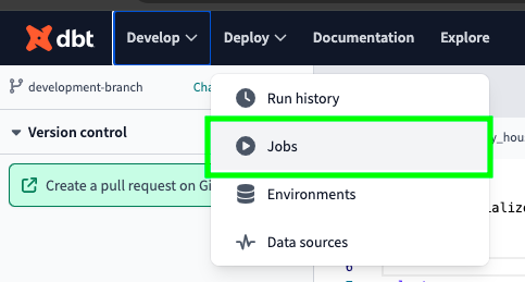
Save the model and push it to production. Now, from the dbt menu, click on Deploy and then on Jobs:

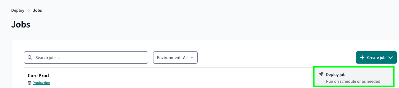
Click on Create job and then on Deploy job:

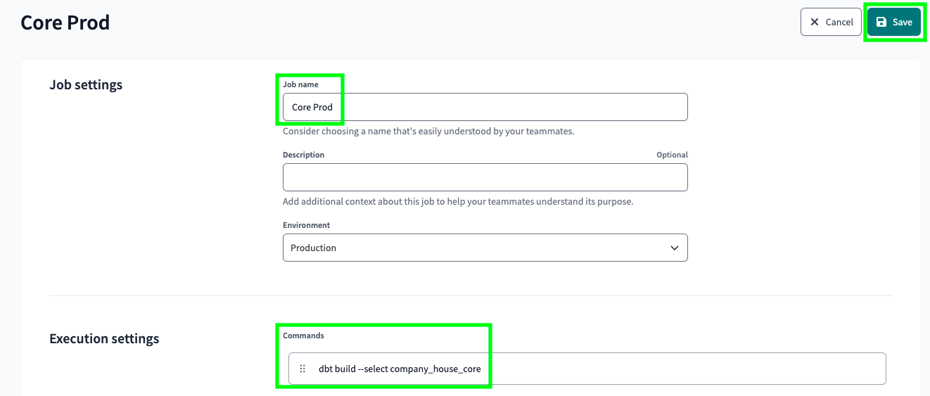
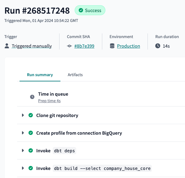
Give a name to your job, add the command dbt build --select company_house_core, which essentially replicates the entire UK’s Companies House data, and click on Save at the top right:

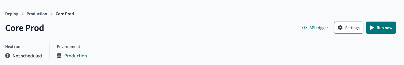
Then, go back to that job and click on Run now at the top right:

Below, at the run history, you can see the current run. Click on it:

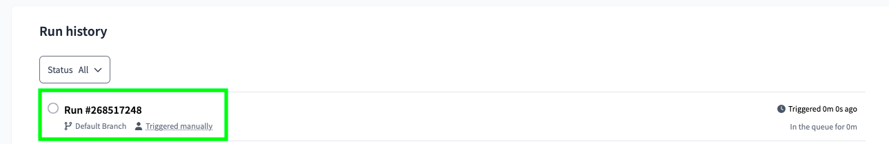
If everything worked correctly, all the steps should be green:

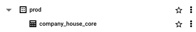
Also, in BigQuery you should see a new dataset named prod with the company_house_core table:

Now, given that our production dataset is called prod, in our configuration environment we need to replace the dataset from dbt_arbenkqiku to prod. Also, I replaced the name of the data sources from development to production:

version: 2

sources:
  - name: staging
    database: streaming-pipeline-418713 # BigQuery project id
    schema: company_house # BigQuery data set
    tables:
      - name: company_house_core
      - name: company_house_stream
  - name: production
    database: streaming-pipeline-418713 # BigQuery project id
    schema: prod # BigQuery data set
    tables:
      - name: company_house_core
      - name: get_last_timestamp
      - name: snapshot_streamed_data

development should be replaced with production in all the models. Also, in the model company_house_core.sql we can replace the code that replicates the entire UK’s Companies House data with the code that merges the most recent streamed data:

As before, commit and sync your changes, create a pull request on GitHub and merge the branches. Remember, if your models are not in the main branch they won’t run in production.

Now, go back to Jobs, and create a job for each model:

• snapshot_streamed_data
• company_house_core_prod. This was already created.
• get_last_timestamp

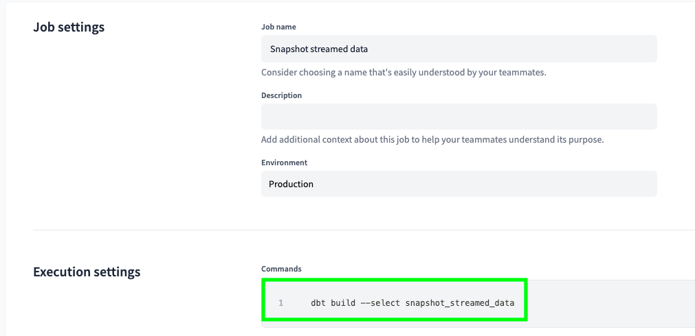
Here is what the job Snapshot streamed data looks like:

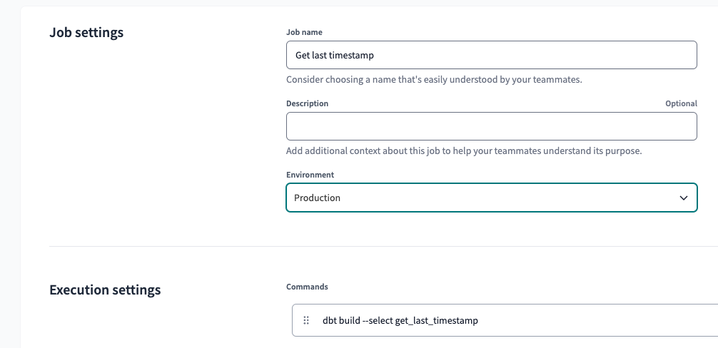
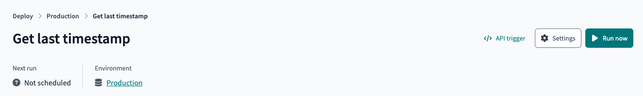
Here is what the job Get last timestamp looks like:

Now, as before, go to the terminal and start the Docker container that produces data to the Kafka topic. When you see production data in the Confluent console, start the Mage streaming pipeline as well. After a couple of minutes, stop these 2 process as we have generated enough new data to test things in our dbt production environment.

Now, let’s run our jobs in the following order:

• Snapshot streamed data
• Core Prod
• Get last timestamp

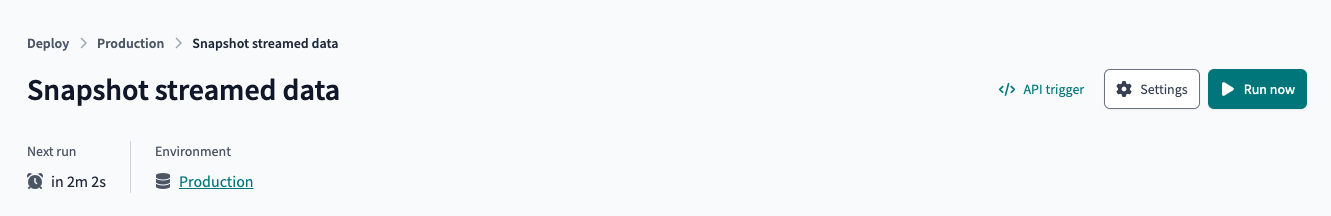
Select the job Snapshot streamed data. Click on Run now:

There should be a new snapshot of data:

Now, select the job Core Prod. Click on Run now:

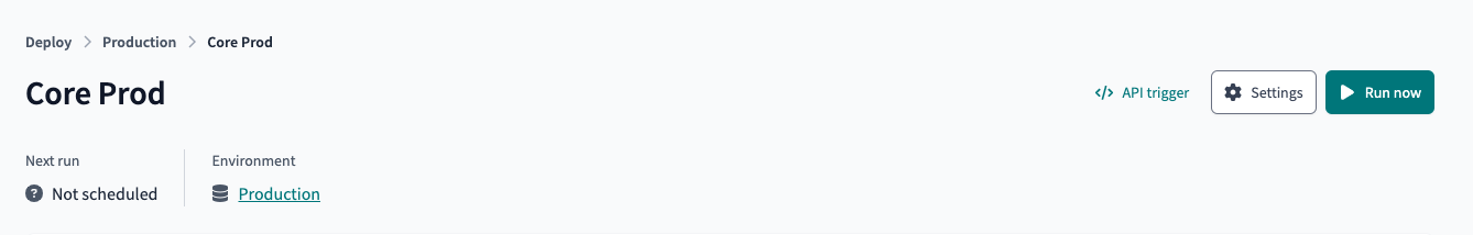
We can see that the data was successfully integrated in the entire UK’s Companies House data:

If we retrieve the most recent timestamp from the snapshot_streamed_data table, we get this

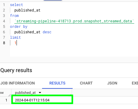
Now, let’s run the Get last timestamp job and see if we get the same result:

Aaaaaaand it matches:

Schedule and Run the Entire Pipeline

Previously, we ran our jobs in the following order:

• Snapshot streamed data
• Core Prod
• Get last timestamp

Now, we need to schedule them. The job Snapshot streamed data, needs to be run separately from the other jobs. This is because we must ensure that the snapshot data remains static and does not change.

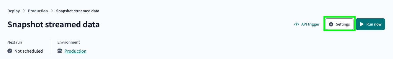
Go to the Snapshot streamed data job and click on Settings:

Click on Edit:

Scroll down, toggle Run on schedule, select Cron schedule and the following Custom cron schedule:

0,20,40 * * * *

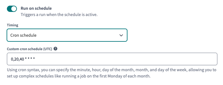
This means that this job will always run at minute 0, 20, and 40 of every hour, every day. Save the job.

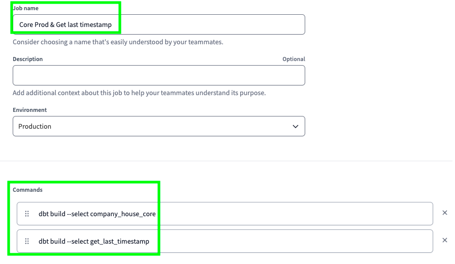
Create a new job named Core Prod & Get last timestamp with the following commands:

dbt build --select company_house_core
dbt build --select get_last_timestamp

Add the following cron schedule:

10,30,50 * * * *

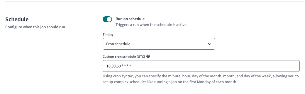
Save the job. On dbt, the maximum frequency for a job is every 10 minutes. Therefore, to test whether everything runs smoothly, we have to be patient.

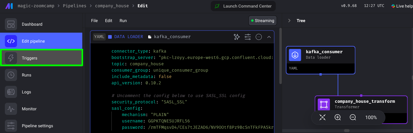
Now, as before, go to the terminal and start the Docker container that produces data to the Kafka topic. When you see production data in the Confluent console, go to Mage and click on Triggers:

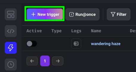
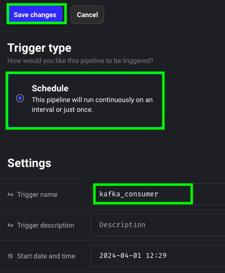
Click on New trigger:

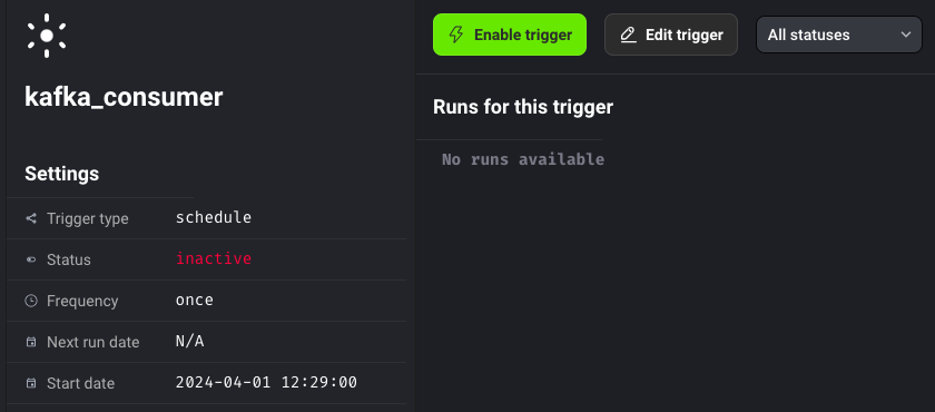
Give a name to the trigger, click on Schedule and then on Save:

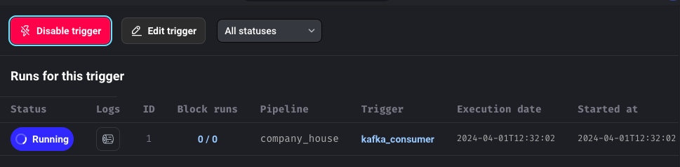
Now click on Enable trigger:

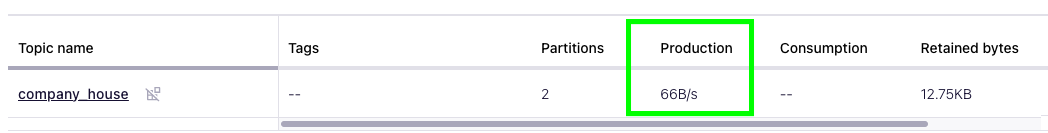
Our pipeline is now running, it consumes data from Kafka and sends it to BigQuery:

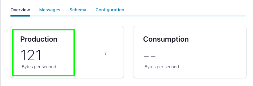
On Confluent, we can see that we’re both producing and consuming 64 bytes per second:

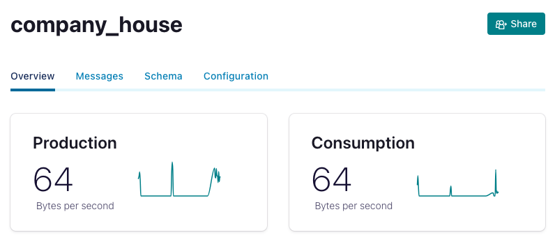
So, I let the entire pipeline run for a couple of hours and no issues were detected. The newly streamed data was successfully integrated into the entire UK’s Companies House data:

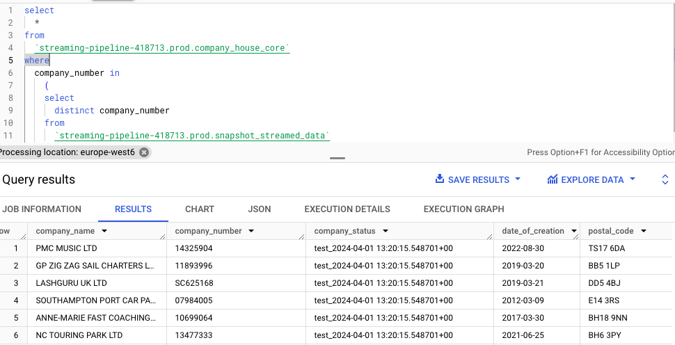
If you recall, in the model snapshot_streamed_data.sql, the column company status was defined as concat("test_", current_timestamp()) as company_status. This was done for testing purposes. Now that we know that everything runs smoothly, we can replace it with simply company_status.