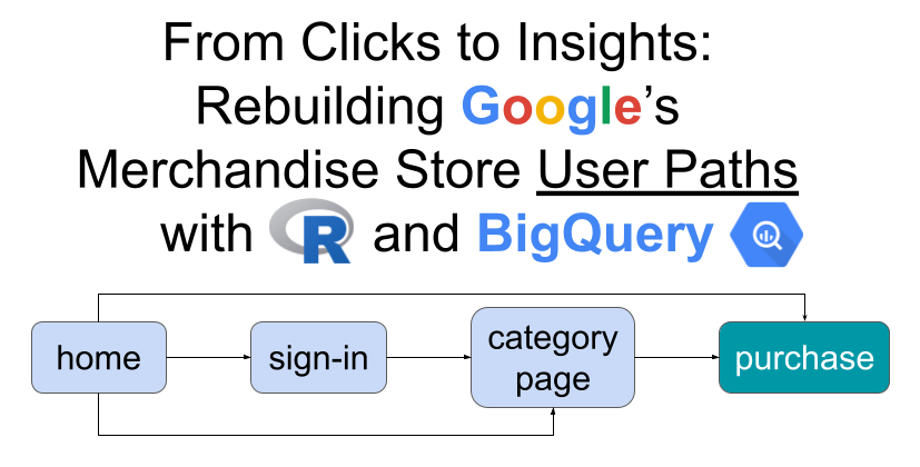
From Clicks to Insights: Rebuilding Google’s Merchandise Store User Paths with R and BigQuery

Table of contents

• What is path analysis?
• What business questions can we answer with path analysis?
• Structure of this article
• What tools are we going to use?
• Extracting data from BigQuery
• Download raw data in R
• Data cleaning
• Data enrichment
• Data analysis
  • Where do users drop off most frequently?
  • What are the most common entry points?
  • Are some landing pages “dead ends”?
  • Funnel analysis by landing pages
  • How do promotion views affect conversion?
  • What happens after users sign in?
• Next steps

What is path analysis?

A user path is the sequence of steps a user takes through your site or product, typically the pages they visit in order, and optionally the events they trigger along the way. Path analysis helps uncover friction points and dark patterns in the user journey.

What business questions can we answer with path analysis?

It is always important to start with business questions so that our analysis brings real value. Here are some possible questions:

• Where do users drop off most frequently?
• What are the most common entry points?
• Are some landing pages “dead ends”?
• How far do users typically progress through the purchase funnel?
• How do promotion views affect conversions?
• What happens after users sign in?

We’ll explore these after cleaning the dataset.

Structure of this article

Some of you might be more interested in the data cleaning and preparation, while others may prefer to jump straight to the analysis and insights. The data cleaning section is intentionally detailed, so if you’re mainly here for the interpretation, feel free to skip ahead to the analysis section.

What tools are we going to use?

We’ll retrieve the raw data with BigQuery and then we’ll build the user paths with R.

You can run path analysis directly in GA4’s Explore section. It’s visually appealing, but the view quickly becomes crowded as it only shows the most frequent paths.

With R, you’re not limited to the top results. You can count every possible path, no matter how rare. You can also mix dimensions, such as combining page location with events, to build a richer picture of user behavior.

For this analysis, we’re going to use Google’s Merchandise Store BigQuery Export. The data is from the 2020-11-01 to the 2021-01-31.

Extracting data from BigQuery

We want to understand how users move through the website and what they actually do once they are there. For this, we are interested in page views and ecommerce events.

Events like “session_start” or “first_visit” don’t tell us much about navigation, so we will exclude them. We also want the results in chronological order, so we can later reconstruct user paths.

Here is the query with comments:

select 
  -- Unique user identifier (anonymous in GA4)
  user_pseudo_id, 

  -- Extract the session_id from event_params
  (select value.int_value from unnest(event_params) where key = "ga_session_id") as session_id, 

  -- The event name (e.g. page_view, purchase)
  event_name, 

  -- Extract the page URL from event_params
  (select value.string_value from unnest(event_params) where key = "page_location") as page_location 

from 
  -- Public GA4 sample ecommerce dataset
  bigquery-public-data.ga4_obfuscated_sample_ecommerce.events_* 

where 
  -- Exclude events that don't describe navigation or user actions
  event_name not in ("session_start", "first_visit", "scroll", "user_engagement") 

order by 
  -- Order events by user, session, and timestamp to reconstruct paths
  user_pseudo_id, session_id, event_timestamp

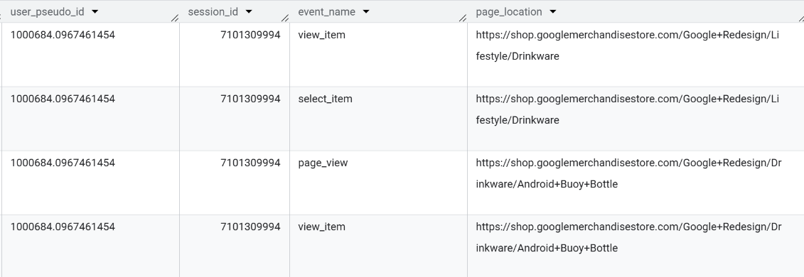
This is the raw data the we’re going to use.

If you would want to learn how to extract data from BigQuery, Simmer offers a great course.

Anyway, let’s save the result as a BigQuery table.

Download raw data in R

Now, let’s download the entire table in R:

# Load libraries
library(tidyverse) # data wrangling and visualization
library(bigrquery) # BigQuery client for R
library(ggrepel) # data viz package
library(scales) # data viz package

# 1 Authenticate to BigQuery with a service account JSON ----
bq_auth(path = "service-account.json")

# 2 BigQuery table reference ----
project_id <- "de-simmer-course-2"
dataset_id <- "articles"
table_id <- "2025_09_29_article_path_analysis_query"

  # download table
bq_table_info <- bq_table(project_id, dataset_id, table_id)
  # bigint = "integer64" preserves large integers (ids, timestamps)
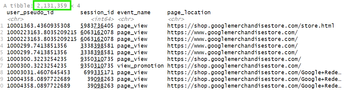
raw_data <- bq_table_download(bq_table_info, bigint = "integer64")

As you can see, our dataset has over 2M+ rows:

Data cleaning

We are only interested in how users navigate between pages, not the full URLs. So we can remove the main domain (for example, “https://shop.googlemerchandisestore.com”) and keep only the path, such as “/home” or “/products”.

raw_data %>% 
  
  # Remove the domain (everything before ".com") from each URL
  # ".*\\.com" = any characters up to and including ".com"
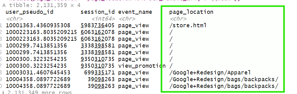
  mutate(page_location = page_location %>% str_remove_all(".*\\.com"))

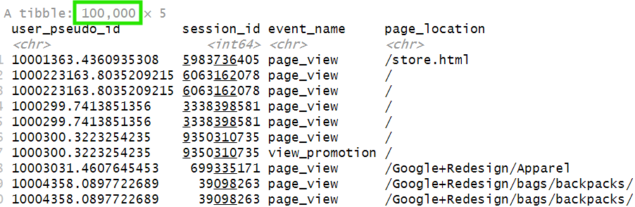
Now the data is easier to read:

Since we’re working with a large dataset, processing can take some time. To test our code more efficiently, we can apply it to only the first 100,000 rows. Once we’re sure everything works as expected, we can then run it on the full dataset.

raw_data %>% 
  
  # select first 100.000 rows
  slice(1:100000) %>% 
  
  # Remove the domain (everything before ".com") from each URL
  # ".*\\.com" = any characters up to and including ".com"
  mutate(page_location = page_location %>% str_remove_all(".*\\.com"))

This returns the first 100,000 rows:

The %>% symbol, known as the pipe operator, lets us chain multiple operations together. It passes the result of one step directly into the next one, so we can apply a new operation to the previous result without creating intermediate variables. In our code, we first select the first 100,000 rows, and then we remove everything before the .com in the page_location column.

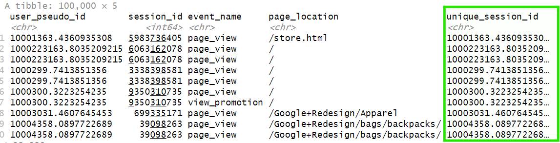
Next, let’s create a unique_session_id column, which is the concatenation of the user_pseudo_id and session_id columns:

raw_data %>% 
  
  # Intermediary code
  
  mutate(unique_session_id = str_c(user_pseudo_id, session_id))

Now we have a new column:

Let’s remove the columns user_pseudo_id and session_id, since they’re no longer needed for the next steps of our analysis.

raw_data %>% 
  
  # Intermediary code
  
  # remove user_pseudo_id and session_id
  select(-user_pseudo_id, -session_id)

Much better:

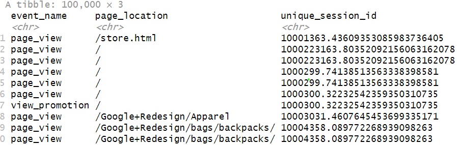
Let’s reorder the columns with unique_session_id first:

raw_data %>% 
  
  # Intermediary code
  
  # reorder columns
  select(unique_session_id, event_name, page_location)

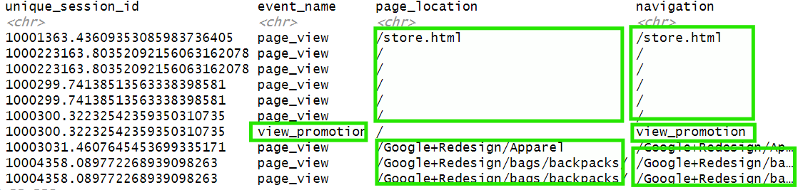
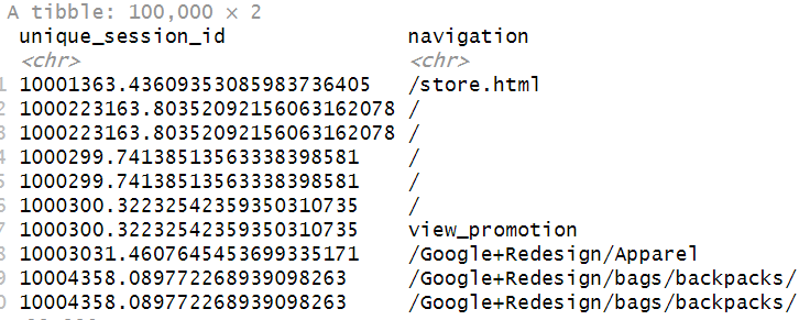
Our goal is to understand which pages users visited and what actions they performed on those pages. To do this, we’ll create a new column that combines both page views and other user events. If the event is page_view, we’ll keep the page URL (page_location) as the value. If the event is something else, like view_promotion or add_to_cart, we’ll use the event name instead.

raw_data %>% 
  
  # Intermediary code
  
  mutate(navigation = case_when(
    event_name == "page_view" ~ page_location,
    TRUE ~ event_name
  ))

The result is a single column that captures both where the user was and what they did there. This navigation column will be key for building the user journey in the next steps, since it merges page views and user actions into a single chronological sequence:

Now, let’s keep only the useful columns, unique_session_id and navigation:

raw_data %>% 

  # Intermediary code
  
  select(unique_session_id, navigation)

These columns are sufficient to build user paths:

Our next goal is to remove duplicate consecutive events. For example, if a user generates two consecutive page_view events on the same page, we want to keep only one of them.

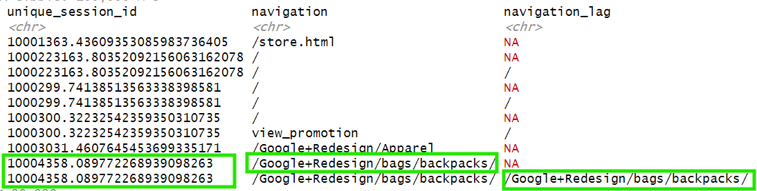
To do this, we first need to compare each event with the one that came before it. For every unique_session_id, we’ll shift the navigation column one step forward to create a new column, navigation_lag.

raw_data %>% 

  # Intermediary code
  
  group_by(unique_session_id) %>% 
  mutate(navigation_lag = navigation %>% lag()) %>% 
  ungroup()

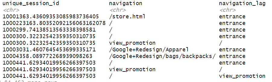
Now, within each unique_session_id, the values of navigation have been moved down one row in the navigation_lag column:

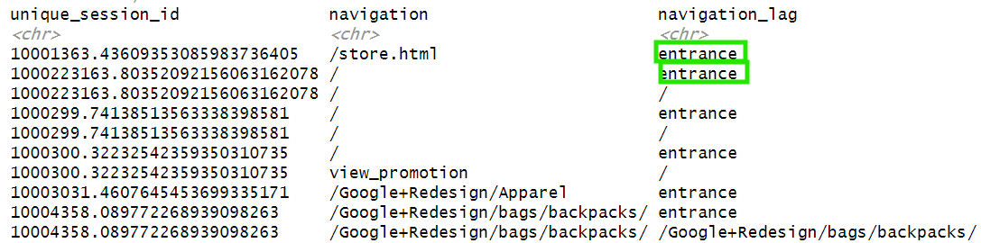
Next, whenever the value in navigation_lag is NA, it means that this was the first page of the session. We’ll label those cases as “entrance” and keep the rest unchanged:

raw_data %>% 

  # Intermediary code
  
  mutate(navigation_lag = case_when(
    is.na(navigation_lag) ~ "entrance",
    TRUE ~ navigation_lag
  ))

This way we have more descriptive values:

Finally, whenever navigation equals navigation_lag, as displayed in the image below:

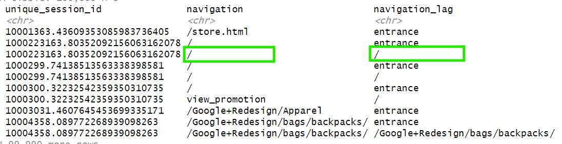
That means the user hasn’t changed page_location, therefore these rows are redundant and we can remove them:

raw_data %>% 

  # Intermediary code
  
  filter(navigation != navigation_lag)

Here is out table without those duplicates:

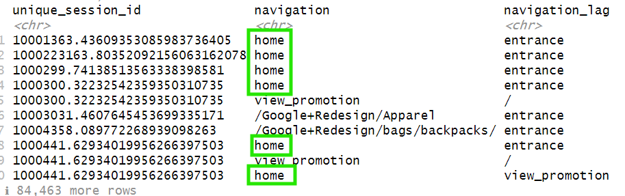
To make the paths more readable, let’s rename “/” or “/store.html” with “home”:

raw_data %>% 

  # Intermediary code
  
  mutate(navigation = case_when(
    navigation %in% c("/", "/store.html") ~ "home",
    TRUE ~ navigation
  ))

Much more readable:

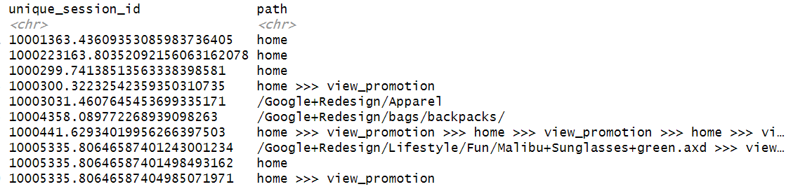
Now, for each unique_session_id, we can combine all navigation steps into a single sequence to represent the user’s full path. Each step will be separated by 3 “>” for readability:

raw_data %>% 

  # Intermediary code
  
  group_by(unique_session_id) %>% 
  reframe(path = paste(navigation, collapse = " >>> ")) %>% 
  ungroup()

Now each row represents the full path of a user:

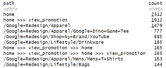
We cannot analyze each row indiviually, so, let’s count how many times all the different user paths occur and order them in descending order:

raw_data %>% 

  # Intermediary code
  
  group_by(path) %>% 
  reframe(count = n()) %>% 
  ungroup() %>% 
  
  arrange(desc(count))

This way we can analyze data more easily:

Now that we’ve confirmed the code works as expected, we can remove the slice(1:100000) line so that it runs on the entire dataset and we can save the result in a variable named paths:

paths <- 

raw_data %>% 

  # Intermediary code
  
  group_by(path) %>% 
  reframe(count = n()) %>% 
  ungroup() %>% 
  
  arrange(desc(count))

Data enrichment

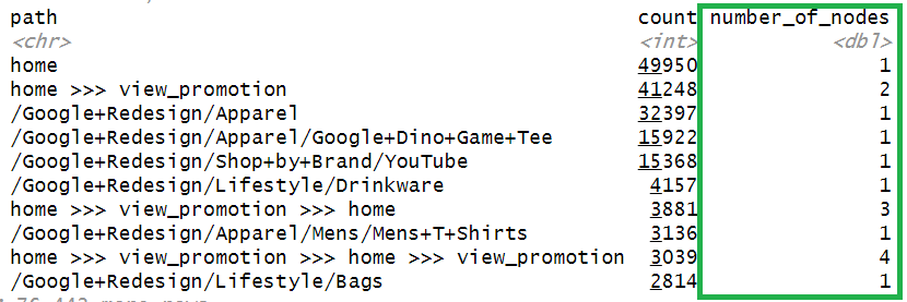
Now that our data is clean, we can actually enrich it. For example, we can count how many nodes each user path contains:

paths_enriched <- paths %>% 
  
  mutate(number_of_nodes = str_count(path, " >>> ") + 1)

This gives additional information to analyze our data:

Data analysis

Where do users drop off most frequently?

To understand where user drop off most frequently, we have to identify the most common exit pages or exit events. Let’s clean the data so we can keep only the last step of each path.

paths_enriched %>% 
  
  # Keep only last step
  mutate(last_step = str_extract(path, "[^>]+$") %>% str_trim()) %>%
    
  # Sum occurence of last step  
  group_by(last_step) %>% 
  reframe(count = sum(count)) %>% 
  ungroup() %>% 
    
  arrange(desc(count))

Here is the count of each exit page or event:

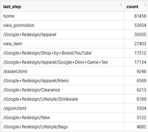
In most user paths, the last step is the home page. This could mean that users return to the home because they can’t find what they’re looking for, or that they leave the website right after arriving. Let’s take a closer look at the paths that end with the home page.

paths_enriched %>% 
  
  # Create last step column
  mutate(last_step = str_extract(path, "[^>]+$") %>% str_trim()) %>%
    
  # Filter paths that end in the home
  filter(last_step == "home")

It seems that a large portion of users exit immediately after landing on the home page.

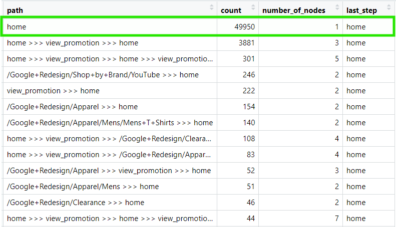
When that happens, it usually means there’s a mismatch between user intent and page content, users didn’t find what they expected. That could point to a targeting issue, where campaigns are driving unqualified traffic. Or it could be a UX problem, where users struggle to navigate or understand what the site offers.

Unfortunately, since this dataset is four years old, we can’t audit the website directly to confirm which is the case.

Another observation: many user paths also end on category or product pages (like /Apparel). That suggests users reach the point of evaluation but not conversion. Possible explanations include:

• Product appeal issues, users aren’t convinced by the offer (price, description, imagery).
• UX issues, product discovery or comparison may be frustrating (filters, sorting, or speed).

Either way, the home and the Apparel category seem like a good starting points for the UX/UI team, as they drive the highest number of exits.

What are the most common entry points?

To get the most common entry points, we must extract the landing page from each user path, namely the first node:

paths_enriched %>% 
  
  # Extract everything before " >>> "
  mutate(landing_page = path %>% str_extract(".* >>>") %>% str_replace_all(" >>>.*", "")) %>%
  
  # If there is only one node, use the path as the landing page
  mutate(landing_page = ifelse(is.na(landing_page), path, landing_page)) %>% 
    
  # Count of landing pages
  group_by(landing_page) %>% 
  reframe(count = sum(count)) %>% 
  ungroup() %>% 
    
  arrange(desc(count)) 

We can see that the home page drives by far the most traffic. After that, most user paths start on product category pages.

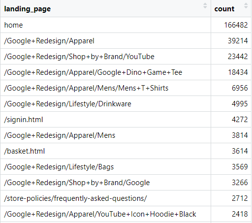
Interestingly, the pages where users enter the website are often the same ones where they leave. A useful next step would be to analyze how far users progress through the website depending on their landing page. Let’s do that.

Are some landing pages “dead ends”?

To understand what landing pages are dead ends, we must extract the average node length by landing page. Also, it is important to weight the node length by user path count.

paths_enriched %>% 
  
  # Extract everything before " >>> "
  mutate(landing_page = path %>% str_extract(".* >>>") %>% str_replace_all(" >>>.*", "")) %>%
  
  # If there is only one node, use the path as the landing page
  mutate(landing_page = ifelse(is.na(landing_page), path, landing_page)) %>% 
  
  # Calculate average weighted node length
  group_by(landing_page) %>% 
  reframe(weighted_avg_nodes = weighted.mean(number_of_nodes, count),
          count = sum(count)) %>% 
  ungroup() %>% 
    
  arrange(desc(count))

Actually, we can see that the home does not perform as bad as the previous analyses would suggest, as the average node length is 6.97.

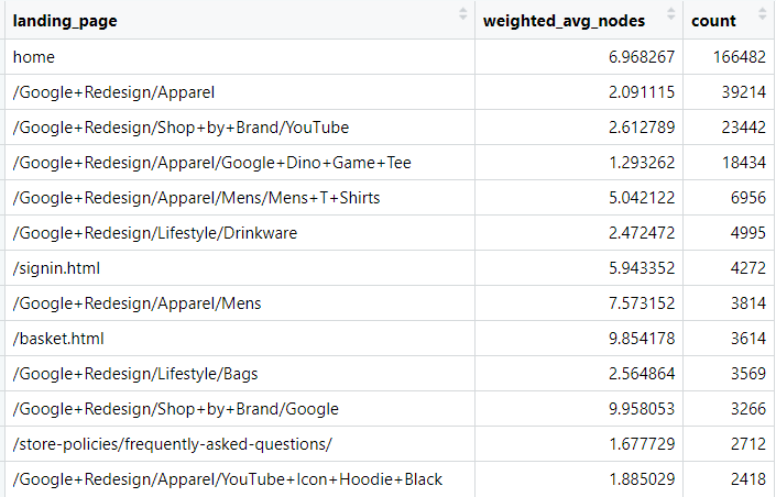
In terms of product categories, we can see that certain categories perform much better than others. For example, Apparel and YouTube categories have 2.1 and 2.6 average node lengths respectively, whereas Mens and Google have 5 and 9.96 average node lengths. So, I would probably urge the UX/UI team to focus on Apparel and YouTube, as they drive a lot traffic, but the average node length is very small.

Funnel analysis by landing pages

Node length is a good indicator, but this doesn’t tell us if users purchase or not. So, to answer that, we can now combine path analysis with funnel analysis. For each landing page, we’ll measure how often key e-commerce events occur, such as view_item, add_to_cart, and purchase, to understand how effectively each entry point drives users through the funnel.

First, let’s extract the landing page from each path, and also whether a path contains a view_item, add_to_cart or purchase event:

paths_with_funnel_steps <- paths_enriched %>% 
    
  # Extract everything before " >>> "
  mutate(landing_page = path %>% str_extract(".* >>>") %>% str_replace_all(" >>>.*", "")) %>%
  
  # If there is only one node, use the path as the landing page
  mutate(landing_page = ifelse(is.na(landing_page), path, landing_page)) %>% 
    
  # Label paths based on view_item event
  mutate(view_item = case_when(
    path %>% str_detect("view_item") ~ "yes",
    TRUE ~ "no"
  )) %>% 
    
  # Label paths based on add_to_cart event
  mutate(add_to_cart = case_when(
    path %>% str_detect("add_to_cart") ~ "yes",
    TRUE ~ "no"
  )) %>% 
    
  # Label paths based on purchase event
  mutate(purchase = case_when(
    path %>% str_detect("purchase") ~ "yes",
    TRUE ~ "no"
  )) 

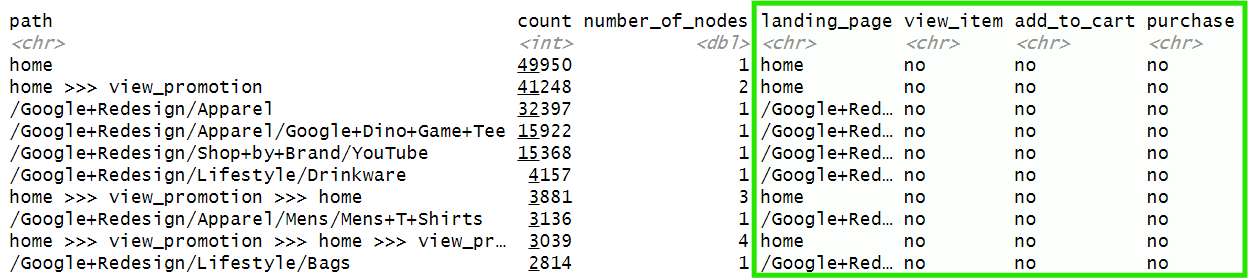
Now each path is correctly labeled:

For each e-commerce event, we’ll calculate the share of paths (per landing page) that contain that event. I’ll refer to this as a “conversion rate” for brevity, but it’s a path-level share, not a session or user conversion rate. Let’s start with view_item event:

view_item_conv_rate <- 
  
  paths_with_funnel_steps %>% 
  
  # Count combinations of landing page and view_item
  group_by(landing_page, view_item) %>% 
  reframe(count = sum(count)) %>% 
  ungroup() %>% 
  
  pivot_wider(names_from = view_item, values_from = count, names_prefix = "view_item_") %>% 
  
  replace(is.na(.), 0) %>% 
  
  # Keep only pages with a significant amount of view item events
  filter(view_item_no > 100) %>% 
  
  # Calculate view item conversion rate
  mutate(view_item_conv_rate = view_item_yes / (view_item_yes + view_item_no)) %>% 
    
  # Sum view item events to get an idea of the importance of each page
  mutate(count = view_item_no + view_item_yes) %>% 
  
  # Select only landing page and view item conversion rate columns
  select(landing_page, count, view_item_conv_rate)

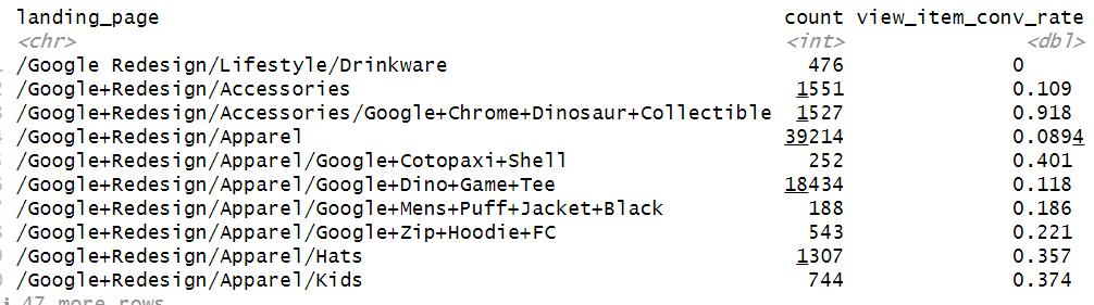
This gives us a table showing how often each page served as a landing page across all paths, along with its corresponding view_item conversion rate:

Let’s do the same for add_to_cart, but let’s filter only the landing pages included in the view_item table we extracted before.

  # landing pages present in view_item table
unique_pages_view_item <- view_item_conv_rate %>% pull(landing_page) %>% unique()

  # add to cart conversion rate by landing page
add_to_cart_conv_rate <- paths_with_funnel_steps %>% 
  
  filter(landing_page %in% unique_pages_view_item) %>% 
  
  # Count combinations of landing page and add_to_cart
  group_by(landing_page, add_to_cart) %>% 
  reframe(count = sum(count)) %>% 
  ungroup() %>%
  
  pivot_wider(names_from = add_to_cart, values_from = count, names_prefix = "add_to_cart_") %>% 
  
  replace(is.na(.), 0) %>% 
  
  # Keep only pages with a significant amount of add to cart events
  filter(add_to_cart_no > 100) %>% 
  
  # Calculate add to cart conversion rate
  mutate(add_to_cart_conv_rate = add_to_cart_yes / (add_to_cart_yes + add_to_cart_no)) %>%
  
  # Select only landing page and add to cart conversion rate columns
  select(landing_page, add_to_cart_conv_rate)

Let’s repeat the same thing for purchase. Finally, let’s join the data:

funnel_steps_joined <- view_item_conv_rate %>% 
  
  left_join(add_to_cart_conv_rate) %>% 
  
  left_join(purchase_conv_rate)

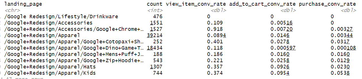
This gives a nice table of all landing pages and their respective conversion rates:

But is difficult to read, so maybe we can create a scatterplot of add_to_cart rate and purchase rate.

funnel_steps_joined %>% 
  
  arrange(desc(count)) %>% 
  
  # Get top 15 landing pages
  slice(1:15) %>%
  
  # Remove basket page
  filter(landing_page != "/basket.html") %>%
  
  # Remove /Google Redesign/ from pages, so that text is more readable
  mutate(landing_page = landing_page %>% str_remove_all("\\/Google\\+Redesign\\/|\\/Google\\ Redesign\\/")) %>% 
  
  # select variables to plot
  ggplot(aes(add_to_cart_conv_rate, purchase_conv_rate)) +
  
  # add coordinates with size based on landing pages count
  geom_point(aes(size = count)) +
  
  # add landing pages to graph
  geom_text_repel(aes(label = landing_page),
                  size = 3) +
  
  # add diagonal line that cuts the plot in 2
  geom_abline(intercept = 0, slope = 0.33, linetype = "dashed", color = "red")+
  
  # change axis labels to percentages
  scale_y_continuous(labels = percent_format()) +
  scale_x_continuous(labels = percent_format()) +
  
  # modify label names
  labs(
    x = "Add to cart conv. rate",
    y = "Purchase rate",
    size = "Count of LPs",
    caption = "Author: Arben Kqiku",
    title = "Conversion rates of top 15 landing pages"
  )

In the chart below, the size of each point represents the number of landing page count, which we can use as a proxy for impact. The red diagonal is a rule-of-thumb baseline relating add to cart conversion rate to purchase conversion rate. Points below the line indicate landing pages where users often add products to their cart but rarely complete the purchase, a sign of friction in the checkout process or weak purchase intent.

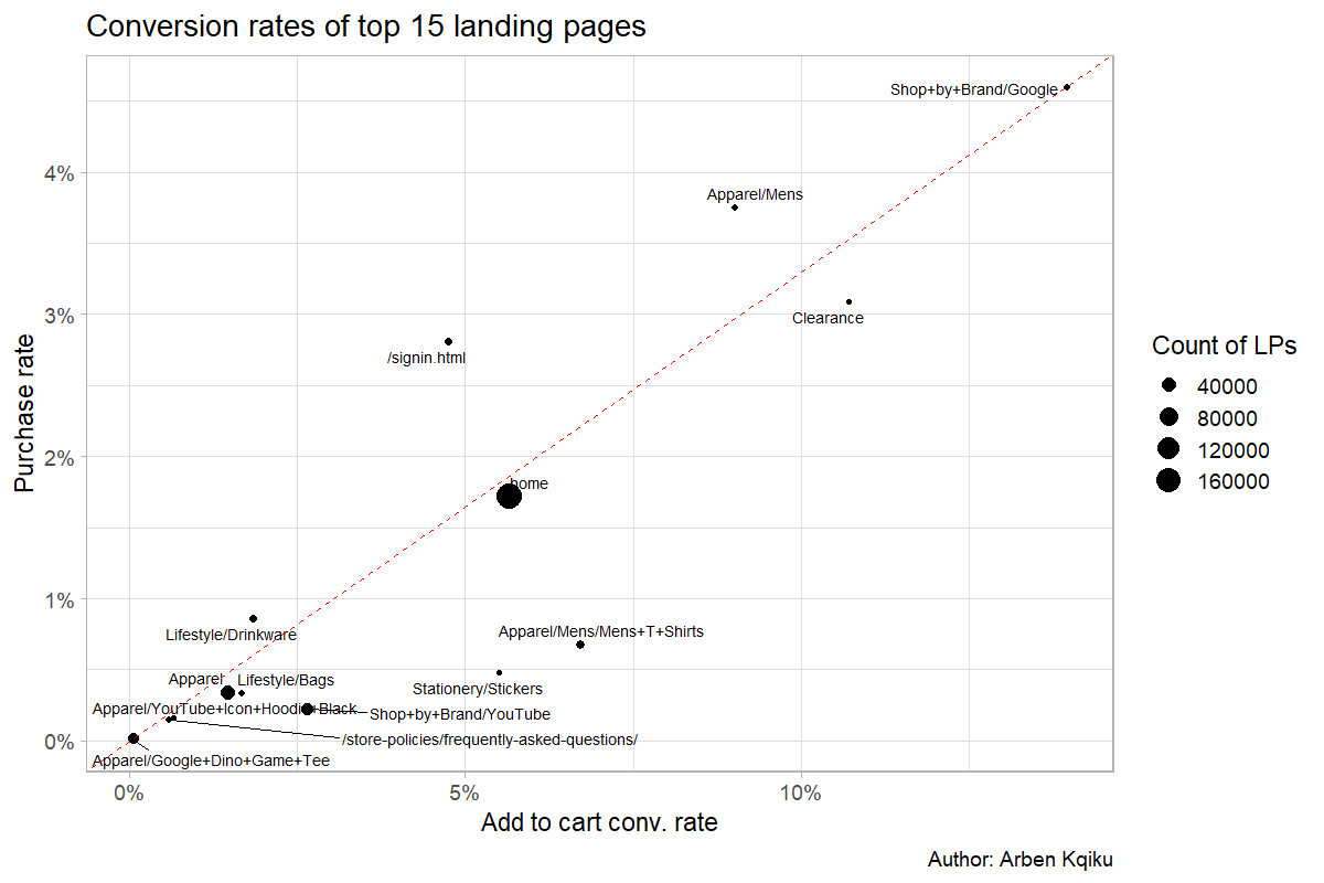
The landing page Apparel/Google+Dino+Game+Tee draws a fair amount of traffic but shows zero add-to-cart and purchase conversions, definitely worth investigating.

Several other pages, such as /Apparel. Lifestyle/Bags, and Lifestyle/Drinkware, have low add-to-cart and purchase rates. If users don’t even add items to their cart, it may indicate a mismatch between their intent and what the page delivers.

The Apparel/Mens/Mens+T+Shirts category drives solid add-to-cart rates but low purchase completion. It could be a logistics issue (e.g., limited shipping regions) or checkout friction. Segmenting by country could help pinpoint the cause.

Finally, Apparel/Mens and Shop+By+Brand+Google are strong performers, efficiently converting add-to-cart events into purchases. If this were live data, I’d explore these pages manually, check search console keywords, and review ad traffic sources to understand what’s driving their success.

How do promotion views affect conversions?

One thing that we can observe from the data is that many user paths include a view_promotion event. So, it would be interesting to understand whether this event leads to a higher conversion rate.

To do that, we have to separate the user paths that contain a view_promotion event from those who don’t, and then, within each group see how many paths contain a purchase event.

paths_enriched %>% 
  
  # Label paths based on view_promotion event
  mutate(paths_with_view_promotion = case_when(
    path %>% str_detect("view_promotion") ~ "view_promotion",
    TRUE ~ "no view_promotion"
  )) %>% 
  
  # Label paths based on purchase event
  mutate(paths_with_purchase = case_when(
    path %>% str_detect("purchase") ~ "purchase",
    TRUE ~ "no purchase"
  )) %>% 
  
  # Calculate combined count of view_promotion and purchase events
  group_by(paths_with_view_promotion, paths_with_purchase) %>% 
  reframe(count = sum(count)) %>% 
  ungroup() %>% 
  
  # Calculate conversion rate
  group_by(paths_with_view_promotion) %>% 
  mutate(conv_rate = count / sum(count)) %>% 
  ungroup() %>% 

  # Extract conv. rate of view promotion Vs. no view promotion
  filter(paths_with_purchase == "purchase") %>% 
  
  select(paths_with_view_promotion, conv_rate)

User paths that include a view_promotion event show a much higher conversion rate (3.3%) compared to those that don’t (0.3%).

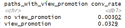
This is a strong signal, but correlation doesn’t imply causation. Are users who were already likely to buy simply more inclined to click on promotions, or do the promotions themselves drive conversions? To find out, we’d need to run an A/B test where one group is exposed to promotions and the other isn’t.

What happens after users sign in?

Let’s filter all paths that include a sign-in event and enrich the data to identify whether those user paths contain a purchase event, whether they start with a sign-in, and what actions follow it.

sign_in_clean <- paths_enriched %>% 
  
  # Filter paths that contain a sign in
  filter(path %>% str_detect("signin")) %>% 

  # Label paths based on whether they start with sign in or not
  mutate(start_with_sign_in = case_when(
    path %>% str_detect("^\\/signin") ~ "yes",
    TRUE ~ "no"
  )) %>% 
  
  # Label paths based on purchase event
  mutate(purchase = case_when(
    path %>% str_detect("purchase") ~ "yes",
    TRUE ~ "no"
  )) %>% 
  
  # Remove the sign in
  mutate(after_sign_in = path %>% str_remove_all(".*\\/signin\\.html")) %>% 
  
  # Keep only the first step after sign in
  mutate(after_sign_in = after_sign_in %>% str_remove_all("^ >>> ") %>% str_remove_all(" >>> .*")) %>% 
  
  # If there is nothing after sign in, label it as an exit
  mutate(after_sign_in = ifelse(after_sign_in == "", "exit", after_sign_in))

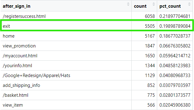
Let’s see what happens after users sign-in:

sign_in_clean %>%  
  
  group_by(after_sign_in) %>% 
  reframe(count = sum(count)) %>% 
  ungroup() %>%
  
  mutate(pct_count = count / sum(count)) %>% 
  
  arrange(desc(count))

We can see that in almost 20% of user paths, users leave the website immediately after signing in. This could point to an issue with the sign-in process itself or a tracking problem. Either way, it’s worth investigating, if this behavior is real, it could represent a significant loss in potential revenue.

How many paths start with a sign in? If we investigate the number of user paths that start with a sign in:

sign_in_clean %>% 
  
  group_by(start_with_sign_in) %>% 
  reframe(count = sum(count)) %>% 
  ungroup() %>% 
  
  mutate(pct_count = count / sum(count)) %>% 
  
  arrange(desc(count))

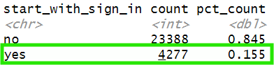
How many paths start with a sign-in? If we look at the data, we can see that 15.5% of all user paths that contain a sign-in event actually begin with one. This strongly suggests a tracking issue, it’s highly unlikely that a user’s first interaction on the site is signing in.

How do user paths that start with a sign-in impact purchases? Let’s combine user paths that start with a sign in with those that contain a purchase event.

sign_in_clean %>% 
  
  # Count user paths that start with a sign in even with purchases
  group_by(start_with_sign_in, purchase) %>% 
  reframe(count = sum(count)) %>% 
  ungroup() %>% 
  
  # Calculate percentage of combination
  group_by(start_with_sign_in) %>% 
  mutate(pct_count = count / sum(count)) %>% 
  ungroup() %>% 
  
  arrange(desc(count)) %>% 
  
  # Remove count column
  select(-count) %>% 
  
  # Turn pct_count into a percentage column
  mutate(pct_count = percent(pct_count, accuracy = 0.1)) %>% 
  
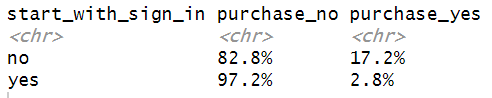
  pivot_wider(names_from = purchase, values_from = pct_count, names_prefix = "purchase_")

Among user paths that begin with a sign-in, only 2.8% lead to a purchase. In contrast, 17.2% of paths that don’t start with a sign-in end in a purchase. This suggests there may be friction in the sign-in process, users could be getting frustrated or encountering an error that prevents them from completing their purchase.

Next steps

Analysis without action is not super useful, so, let’s end this article with some recommendations:

• Run an A/B test on promotions. User paths with a view_promotion event show much higher purchase conversion rates. Testing can confirm whether the promotion itself drives this effect.
• Fix potential sign-in issues. Paths starting with a sign-in have significantly lower purchase rates, suggesting friction or tracking loss.
• Investigate the landing page Apparel/Google+Dino+Game+Tee. It receives notable traffic but has zero add-to-cart and purchase conversions.
• Review /Apparel, Lifestyle/Bags, and Lifestyle/Drinkware. Low engagement on these pages could stem from a mismatch between user intent and landing-page content. If targeting is correct, assess UX and layout.
• Segment Apparel/Mens/Mens+T+Shirts by country. Strong add-to-cart rates but weak purchases may reflect logistics limits such as restricted shipping.
• Analyze traffic sources for Apparel/Mens and Shop+By+Brand+Google. Both convert efficiently; understanding which channels drive them could inform campaign scaling.

If you enjoyed this article, connect with me on LinkedIn.

Happy coding :)